Discrete & Continuous Time: Concepts, Models, & Interpretations

Last updated on Oct 28, 2019 13 min read autoregressive models, time based modeling, dynamical systems, R

Introduction

The page was originally made for Jonathan Butner’s Dynamical Systems Modeling for the Social Sciences class, Spring 2018, University of Utah. This webpage will serve as an introduction to handling of time in dynamical systems models. Mainly, we will focus on how change over time models can be conducted simply as a series of regressions in base R, linking these models to different notions of time. Lastly, we will briefly present some more advanced methods for estimating continuous time models using derivatives, both using observed variables and a latent variable approach.

Our goal throughout this webpage is to provide a link between dynamical systems concepts of time, implementation of models using code, and easily-digestible interpretations of discrete vs continuous time models. We highly recommend basic familiarity with dynamical systems concepts and models to get the most out of this webpage. Jonathan Butner’s Dynamical Systems for the Social Sciences book is an extremely helpful resource, and we would recommend basic familiarity with the concepts he covers in chapters 1-4. For additional information and citation of methods/ideas, please see the reference section.

Download code used for this post.

Discrete and Continuous Time (flow) in Dynamical Systems

Dynamical systems theorists are primarily focused on changes over time. But the conceptualization of time is not often straightforward and involves a conscious decision by a researcher as to how to treat time in dynamical systems models. The purpose of this page is to describe how time is handled in dynamical systems both qualitatively and quantitatively. Primarily we will focus on the difference between discrete and continuous time. R code and examples will be provided to assist all those interested in implementing different models of time. First, let’s describe how we can conceptualize time.

What is time? Does time flow forward? Well, really only experientially. Mathematically, it can be described as a measure of matter’s movement through space. Sorli and Klinar(2007), suggest that time as we experience it may be best thought of as a numerical order of matter’s position. Thus, what we experience is matter at position x1, and then x2, and x3, and so on, not matter flowing through time. One way to imagine this is by thinking about flip books.

A flip book usually has many pages showing an object or scene, such as ball, in slightly different locations on each page. Then, when we quickly flip through the pages, it looks like the ball is moving, perhaps bouncing. Flip books capitalize on how the visualize system processes information. Similarly, we experience a flow of time, because matter is in constant motion.

This phrase sums up Sorli and Klinar’s position fairly well and much better than we can do here: >“Time is a stream of numerical order of motion of [matter] into a-temporal space.” And this distinction is important. Mathematical time vs. Perceived time (for additional information and insights, see McGrath & Kelly, 1986, chapter 2).

Time is constant, right? Well, kind of. Time dilation, or the slowing of passage of events is possible. The classic twin paradox, a problem concerning special relativity, exemplifies this in terms of physics. In it, one twin makes a round trip into space going extremely fast, while the other twin stays on Earth. Although both twins are moving through space, the twin in space (who is moving faster) ages less than the twin who remained on Earth.

Although this is fascinating, the point here is to demonstrate that time, in mathematics, is much more malleable than we might think. How does this apply to dynamical systems?

As you may recall, dynamical systems approaches are interested in change over time. But before we add time, let’s talk about simple positions. As mentioned above, we can think of the movement of an object in terms of positions. Please note, this description was motivated by Gottman’s (2002, chapter 4) description of position using the example of (Winnie the) Pooh sticks. We can highly recommend this chapter as an excellent and simple refresher on limits and derivatives.

Let’s imagine we are interested the relation between state anxiety (x-axis) and frequency of tweets (y-axis). We might assume that some people who experience higher state anxiety tweet more. What we are describing is a simple linear relation between two variables. Further, time is not necessary to describe position. However, if we want to embed the notion of time into our examination we can look at the change from one position to the next (i.e., rise/run or slope). Slope gives us information about change in position from point A to point B and in Šorli and Klinar’s words, we are describing the relation of motion in the stream of numerical order.

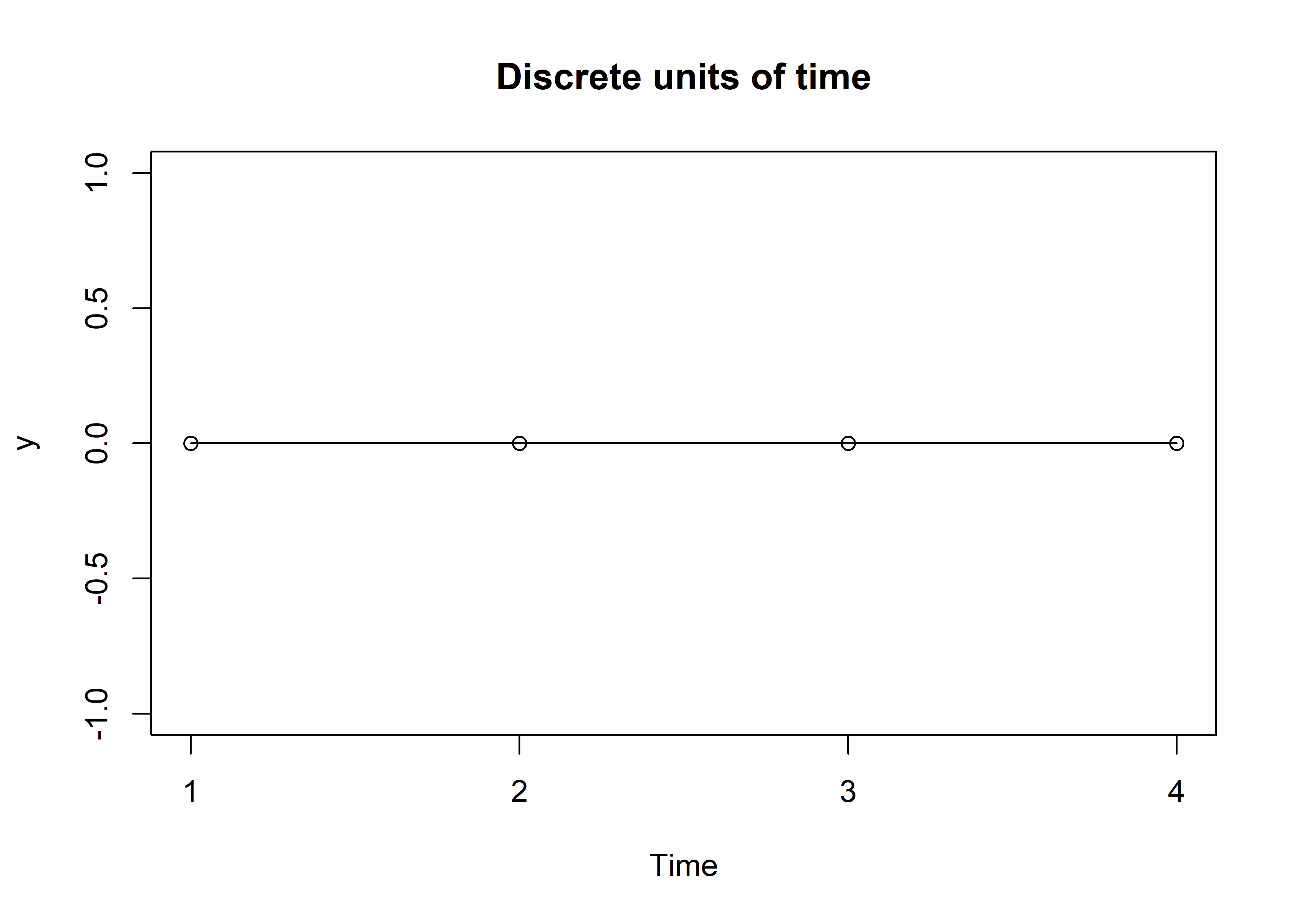
As mentioned above, time can be conceptualized as discrete or continuous. For example, if we imagine a stationary variable at time 1 (t1), t2, t3, and t4 we can think about how at each time, we have a specific break-point. In the graph below, the dots would represent those break-points.

x <- c(1, 2, 3, 4)
y <- c(0, 0, 0, 0)
marks <- c(1, 2, 3, 4)

plot(x, y, xaxt = "n", 
     xlab='Time', 
     main = "Discrete units of time") + 
  lines(x, y) + 
  axis(1, at = marks, labels = marks)

## numeric(0)

Each break point would be a discrete unit of change. This makes fairly logical sense when we think about how we typically measure something like anxiety over time. For example, we might ask someone over a span of 4 days what their peak state anxiety was. We assume continuity in time, but we (mathematically) handle it as discrete units.

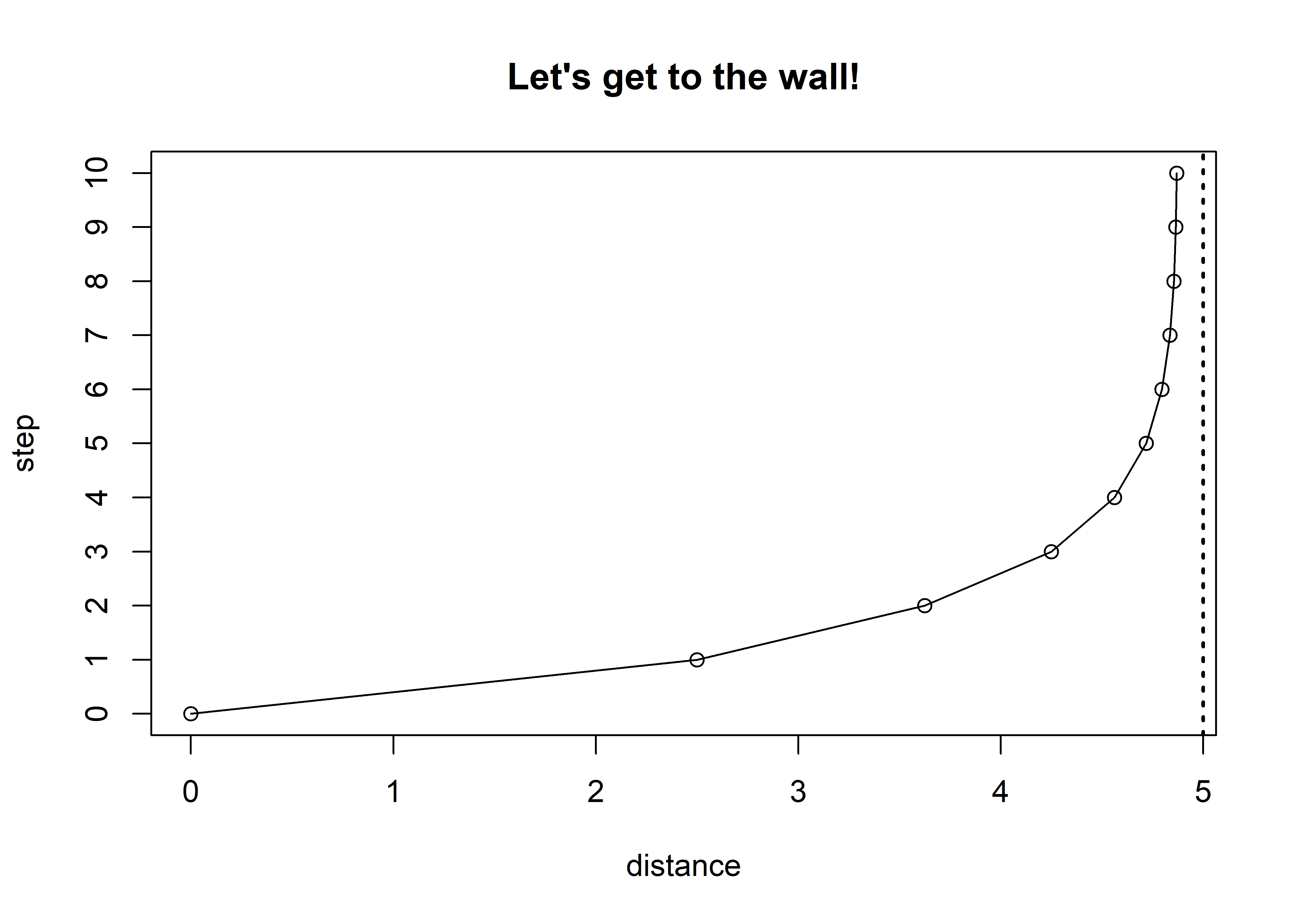
Continuous time on the other hand requires an understanding of limits. Limits can be defined as “a value to which a function or sequence tends as time gets very large” (Gottman, 2002, p. 51). An easy way to understand limits is to imagine standing 5 ft from a wall. Your goal is to get to the wall, but you can only take a step that is half of the total distance from you to the wall. So, when we started, we were 5 ft from the wall, our first step would be ½ the distance (i.e., 2.5 ft), our next step would be half the distance or ¼the initial distance (i.e., 1.25 ft), and so on. What you would notice is that we would actually never reach the wall. But what you also probably reasoned was that we would get so close to the wall it wouldn’t really matter, our location would be indistinguishable from the wall’s location.

distance <- c(0, 2.5, 3.625, 4.25, 4.5625, 4.71875, 4.796875, 4.835938, 4.855469, 4.865235, 4.870118)
step <- c(0, 1, 2, 3, 4, 5, 6, 7, 8, 9, 10)

df <- data.frame(distance, step)

plot(distance, step, 
     main = "Let's get to the wall!", 
     ylim=c(0, 10)) + 
  lines(smooth.spline(distance, step)) + 
  axis(side=2,at=seq(0,10,1)) + 
  abline(v = 5, lty = 3, lwd = 2)

## numeric(0)

Ultimately, your decision about whether to handle time as discrete or continuous is mostly driven by how you want to conceptualize your data, but can lead to differences in interpretation. Below are examples of how one might handle time as discrete or continuous.

Discrete Time: Autoregressive models

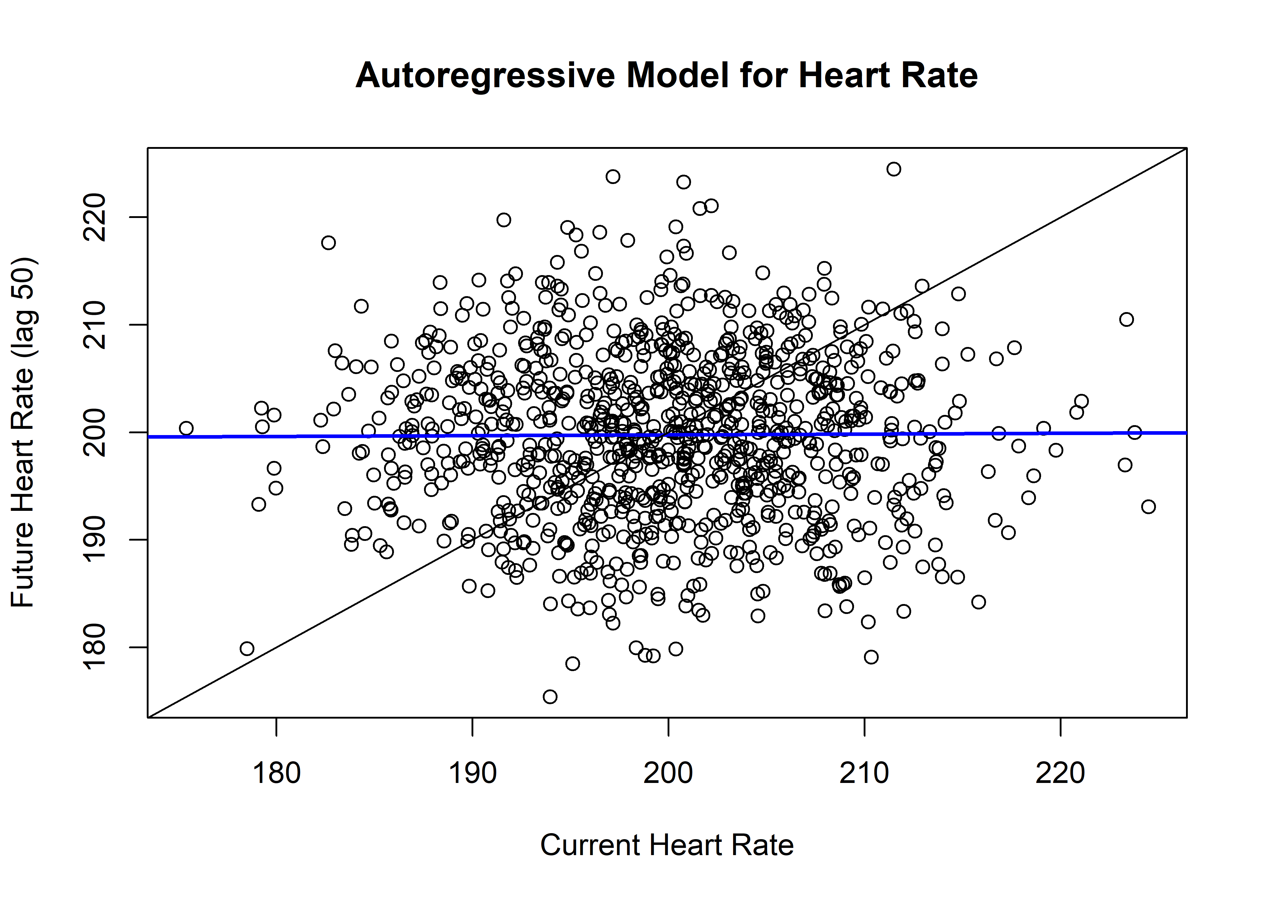
Now, we will read in datafile and clean up the datafile a little bit. We will simulate a random data set of 1000 observations, imagine this is a physiological measure of heart rate related to anxiety throughout the examples. For the autoregressive model, we will be plotting our heart rate variable against itself at some future time, which allows us to see how our current heart rate predicts our future heart rate.

require(Hmisc) #for easily making lags and leads in your data
set.seed(999)
anxiety <- as.data.frame(filter(rnorm(1000, 200, 8), 
                                filter=rep(1,1), 
                                circular=T)) #simulate gaussian noise stationary time series 

colnames(anxiety) <- c("HR")
anxiety$HR <- as.numeric(anxiety$HR)

anxiety$HRlag <- as.numeric(Lag(anxiety$HR, 50)) #where the second number indicates amount to lag by. Note you can also use negative numbers, such as -1, to indicate a lead variable. Usually you'll want to assign this to a new variable so you don't lose your original data.

anxiety$HRlead <- as.numeric(Lag(anxiety$HR, -50)) #lets create a lead as well. 

attach(anxiety)
plot(HRlead, HR,main = "Autoregressive Model for Heart Rate", 
     xlab = "Current Heart Rate", 
     ylab = "Future Heart Rate (lag 50)") + 
  abline(a = 198.204993, b = 0.007827, 
         col = "blue", lwd = 2) + 
  abline(a = 0, b = 1)

## integer(0)

The crossing of the blue line over the reference line indicates the dynamic pattern in your system of interest. In autoregressive models, when the slope is between -1 and 1, that indicates that there is an attractor. In otherwords, heartrate is generally hanging around the crossing point, or set point, somewhere around 200 beats.

Discrete Time: Difference models

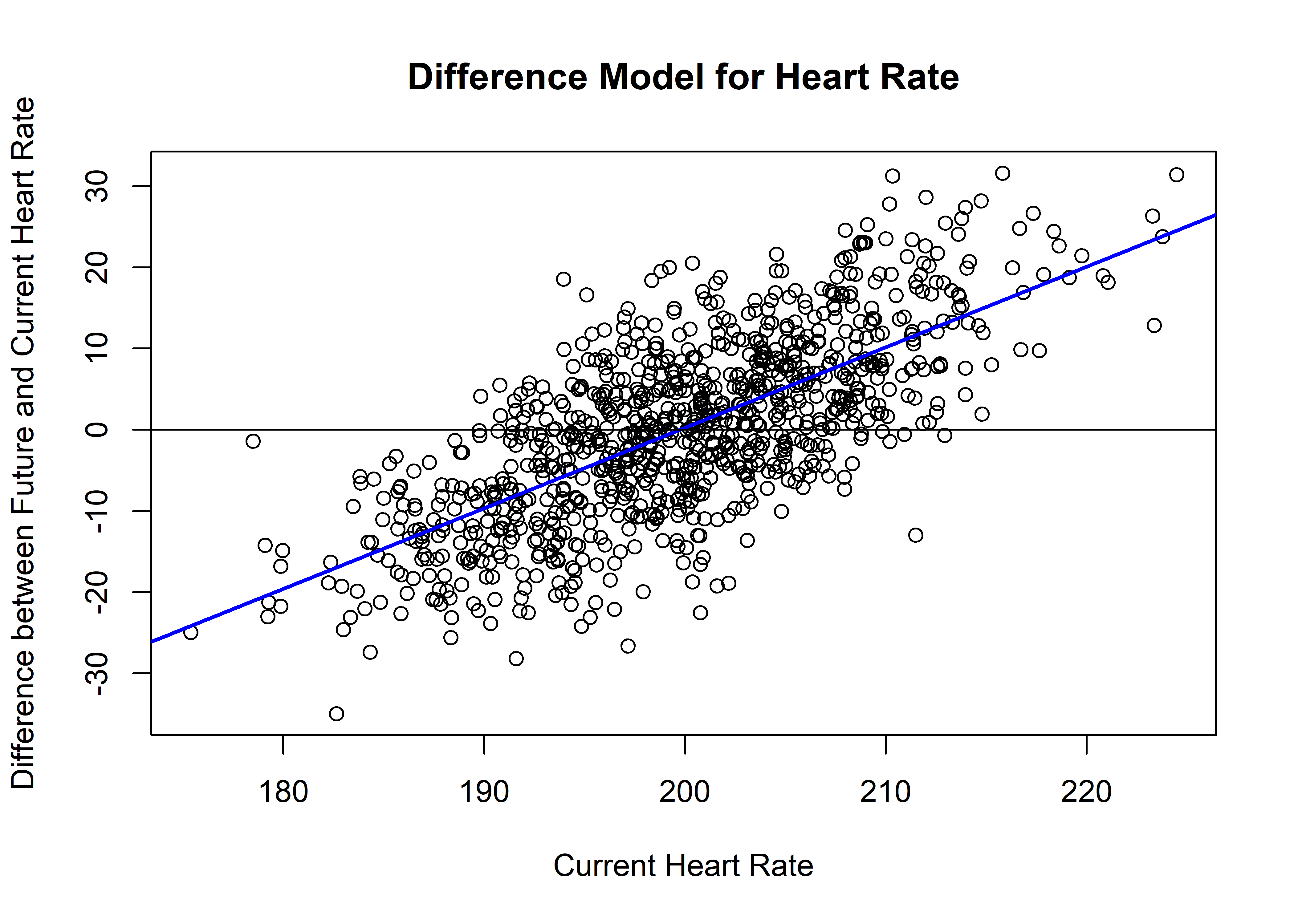
The leap to difference models is not a hard one to make in code, but involves a different way of thinking about time which will affect how we interpret the results of our models. The difference model approach takes the autoregressive lead/lag approach one step further, where you must create a new “difference” variable by taking the difference between your lag variable and your original variable.

anxiety$HRdiff <- anxiety$HR - anxiety$HRlag

plot(anxiety$HR, anxiety$HRdiff, 
     main = "Difference Model for Heart Rate", 
     xlab = "Current Heart Rate", 
     ylab = "Difference between Future and Current Heart Rate") + 
  abline(a = -198.20499, b = 0.99217, 
         col = "blue", lwd = 2) + 
  abline(a = 0, b = 0)

## integer(0)

As you can see, our visualizations of the data are different and so too is our interpretation of the slope of the line crossing the reference line. On the y-axis, we have values indicating points of no change (or where there is no difference between current and future heart rate). Here we see a slope of around 1. According to Butner (2017), in difference score approaches, a slope that is greater than 0 is actually indicative of a repellor.

Continuous Time: Differential Estimation Approaches

Another way of conceptualizing time is in a continuous notion - where we imagine time flowing to, but never reaching infinity, across all possible values of time, as we mentioned in the introduction earlier. Note that although continuous time approaches are widely used by systems theorists, discrete models are still valid.

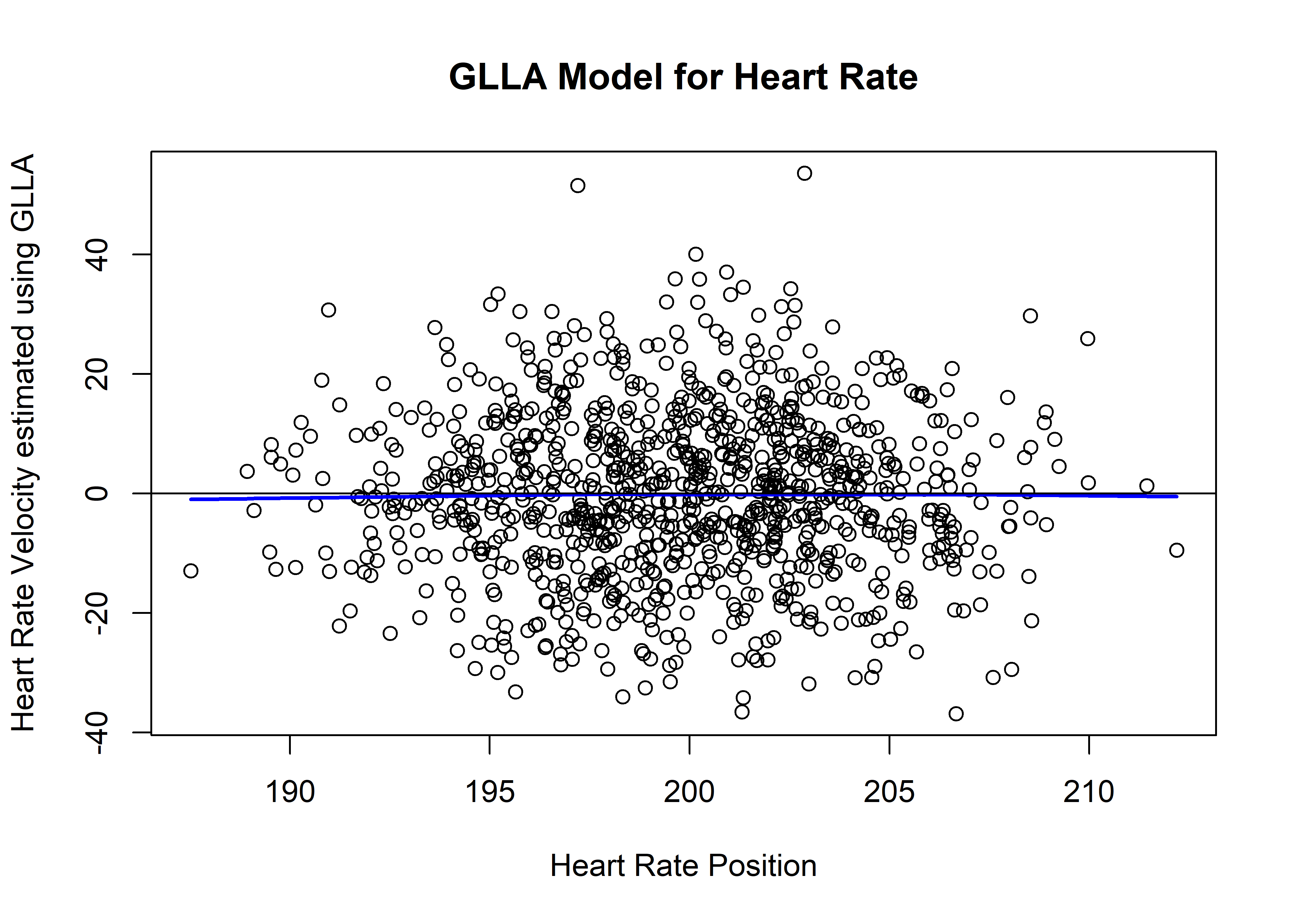
A first method for conceptualizing continuous time is referred to as generalized local linear approximation (GLLA). GLLA essentially attempts to estimate a series of straight lines through your data in order to best approximate velocity. Code for implementing the GLLA function on your own data is provided below, if it is used, please provide attribution to Boker, Deboeck, & Keel (2010).

Embed <- function(x,E,tau) {
  len <- length(x)
  out <- x[1:(len-(E*tau)+tau)]
  for(i in 2:E) { out <- cbind(out,x[(1+((i-1)*tau)):(len-(E*tau)+(i*tau))]) }
  return(out)
}

GLLA <- function(x, embed, tau, deltaT, order=2) {
  L <- rep(1,embed)
  for(i in 1:order) {
    L <- cbind(L,(((c(1:embed)-mean(1:embed))*tau*deltaT)^i)/factorial(i))
  }
  
  W <- solve(t(L)%*%L)%*%t(L)
  EMat <- Embed(x,embed,1)
  Estimates <- EMat%*%t(W)
  
  return(Estimates)
}

Function code details:

GLLA(x, embed, tau, deltaT) x=time series

embed=values that correspond to the number of observations and time interval in the embedded matrix. For example 5 will produce an embedding dimension of 5, with equally spaced intervals of 1 unit of time.

tau= only useful if you want to do something like use every-other-observation. Otherwise use 1. 2 will use every other observation, 4 every 4th observation, etc.

deltaT= time between obs where you must consider your time unit. So if your time unit is seconds, and you sampled 4 times a second, your deltaT should be .25. If your time unit is months and you sampled 4 times a month, your deltaT should be .25.

order= max order of derivative to estimate. 1=velocity (1st derivative); 2=acceleration (2nd derivative). We will use velocity in this example.

This will probably make more sense with an example of the function in action - below we provide an example of using using GLLA to estimate a derivative from the simulated heart rate data.

GLLAHR <- GLLA(x=anxiety$HR,
               embed=4,
               tau=1, 
               deltaT = .25, 
               order=1) #makes new dataframe with original variable (HR) as first column, and 1st order derivative (velocity) as second column
GLLAHR <- as.data.frame(GLLAHR) #make into dataframe
colnames(GLLAHR) <- c("HRposition", "HRvelocity") #rename columns for ease of tracking variables

plot(GLLAHR$HRposition, GLLAHR$HRvelocity, 
     main = "GLLA Model for Heart Rate", 
     xlab = "Heart Rate Position", 
     ylab = "Heart Rate Velocity estimated using GLLA") + 
  lines(lowess(GLLAHR$HRposition, GLLAHR$HRvelocity, 
               f = 50, delta = 10), col = "blue", lwd = 2) + 
  abline(a = 0, b = 0) #plot results

## integer(0)

Next, we provide code for the Generalized Orthogonal Derivative Estimates (GOLD) method. The primary difference between the GOLD method and the GLLA method is the method of estimation used for the derivative. See Hunter (2016) for more on the differences between GLLA and GOLD in a simulation study. Note if you use the GOLD method, be sure to cite Deboeck (2010), who generated this code.

Function code details:

GOLD(x, Time, max,tau) x=time series

Time=values that correspond to the number of observations and time interval in the embedded matrix. For example 1:5 will produce an embedding dimension of 5, with equally spaced intervals of 1 unit of time.

Max= max order of derivative to estimate. 1=velocity (1st derivative); 2=acceleration (2nd derivative). We will use velocity in this example.

tau= only useful if you want to do something like use every-other-observation. Otherwise use 1. 2 will use every other observation, 4 every 4th observation, etc.

Implementation of GOLD in R mirrors the impementation of GLLA outlined previously, substituting the GOLD function for the GLLA function to estimate a derivative from the simulated heart rate data.

GOLD Function

 ContrastsGOLD <- function(Time,max) {
         Xi <- matrix(NA,max+1,length(Time))
       	  	for(r in 0:max) {
          	    	Xi[r+1,] <- (Time^r)
          	    	if(r>0) {
                   	for(p in 0:(r-1)) {
                       	 Xi[r+1,] <- Xi[r+1,] -
                      	       (Xi[p+1,]*(sum(Xi[p+1,]*(Time^r)))/(sum(Xi[p+1,]*(Time^p))))
                       	 }}}
         DXi <- diag(1/factorial(c(0:max)))%*%Xi
	 	 t(DXi)%*%solve(DXi%*%t(DXi))
         }
    
	GOLD <- function(x, Time, max,tau) {
          W <- ContrastsGOLD(Time,max)
          X <- Embed(x,length(Time),tau)
          Est <- X%*%W
          return(Est)          
          }
         
    Embed <- function(x,E,tau) {
         len <- length(x)
         out <- x[1:(len-(E*tau)+tau)]
         for(i in 2:E) {
              out <- cbind(out,x[(1+((i-1)*tau)):(len-(E*tau)+(i*tau))])
              }
         return(out)
         }

Continuous Time: Unobserved Latent Variable Approach using SEM

Though it is beyond the scope of this page, there are also methods allowing for latent variable estimations of derivatives. These methods are beyond the scope of this webpage, but can be implemented using the lavaan package in R for structural equation modeling (Rosseel, 2012). We highly recommend Newsom’s (2015) book describing these techniques, along with other longitudinal modeling techniques using structural equation modeling approaches.

Summary

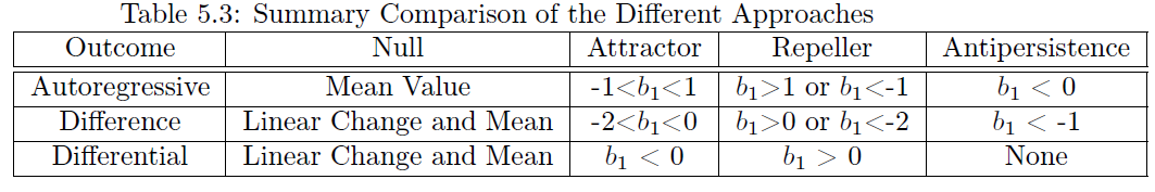
In this webpage, we have tried to provide simple conceptual and coding examples of discrete time (difference and autoregressive approaches) and continuous time (observed differential and latent differential, albeit briefly for the latter). The helpful figure below from Butner helps to briefly summarize the interpretation differences between each approach, if you are familiar with the language of topology (attractors and repellers).

Table adopted from Butner (2017) relating each time modeling approach to topology and associated interpretations.