Checking the Assumptions of Linear Regression
Table of Contents
Introduction
This tutorial will help you test major assumptions of linear regression using R. The tutorial assumes that you have some familiarity understanding and interpreting basic linear regression models already. Meeting the assumptions of regression is important since regression coefficients, standard errors, confidence intervals, and significance tests can be biased when these assumptions are violated. This results in researchers making unfounded or exaggerated claims based on their regression models, which in turn leads to replication issues. Note, however, that regression is generally robust to minor violations of these assumptions (Cohen, Cohen, West, & Aiken, 2003). After going over the assumptions of regression, I’ll review outlier detection and removal, since outliers can greatly skew significance tests. Lastly, I include two functions that quickly check a subset of regression assumptions. Note that clicking these links will reference you to the appropriate sections on this page.
Our example experiment involved collecting a measure of self-reported state fear and a measure of self-reported state fear. We then asked participants to provide a height estimate for a vertical height. We were interested in asking whether state or trait fear more heavily influence perceptual height judgments. Thus, we decided to run a 2-predictor regression. We will be working with a dataset for 25 participants. Note that the state fear and trait fear variables have been mean-centered to make the regression intercept interpretable, since no participants had a state or trait fear value of 0 and the scale for each is interval. Feel free to download it from my website if you want to work with it directly or try any of the examples laid out in the tutorial in R. In addition, you may also want to use your own dataset in R - simply substitute your dataframe, variable, and column names in the code where appropriate.
Download code used for this post.
Major assumptions of regression
Seven Major Assumptions of Linear Regression Are:
The relationship between all X’s and Y is linear. Violation of this assumption leads to changes in regression coefficient (B and beta) estimation.
All necessary independent variables are included in the regression that are specified by existing theory and/or research. This asusmption serves the purpose of saving us from making large claims when we simply have failed to account for (a) better predictor(s) which may share variance with other predictors. Obviously, the regression interpretation becomes extremely difficult and timely once too many variables are added to the regression. We must balance this with accurate representations of population-level phenomena in our model, so usually we would like to test more than one predictor if possible. This will not be covered in this tutorial as meeting this assumption is up to your discretion as a researcher, dependent on knowledge of your specific research topic and question.
The reliability of each of our measures is 1.0. This assumption is almost always violated, particularly in psychology and other fields that generate their own scales, including measures of self-report. Typically, a reasonable cutoff is considered a reliabilty of .7. This will typically downward bias (make smaller) the regression coefficients in your model. This will not be covered in this tutorial as meeting this assumption is nearly impossible and reliability/psychometrics stand on their own as an entire topic of statistical study.
There is constant variance across the range of residuals for each X (this is sometimes referred to as homocedasticity, whereas violations are termed heteroscedastic).
Residuals are independent from one another. Residuals cannot be associated for any subgroup of observations. This assumption will always be met when using random sampling in tandem with cross-sectional designs. This refers to dependencies in the error structure in of model. In other words, there can be no data dependencies, such as that which would be introducted from nested designs. Multilevel modeling is a more appropriate generalized form of regression which is able to handle dependencies in model error structures (for more on multilevel modeling as a regression technique, see Raudenbush & Bryk, 2002).
There is no multicollinearity (a very high correlation) between X predictors in the model. Violation of this assumption reduces the amount of unique variance in X that can explain variance in Y and makes interpretation difficult.
First, we’ll load required packages, read-in the datafile, and assign the regression to a new object.
##this calls the packages required. use install.packages('packagename') if not installed. We will focus on using ggplot2 for plotting, along with an extension GGally, car, and MASS for outlier detection.
library(ggplot2)
library(GGally)
library(car)
library(MASS)
feardata <- read.csv('feardata.csv') #read-in datafile
fit <- lm(HeightEstimate ~ StateFear_c + TraitFear_c,feardata) #assign regression results to fit
Great, so now that we have our dataset and model read into the R environment, we can move forward to checking the first assumption of linearity.
Checking the assumption of linearity
theme_set(theme_bw(base_size = 12)) #changes default theme to black and white with bigger font sizes
ggpairs(feardata, columns = 7:5) #this will create a scatterplot matrix of each of our X variables (trait and state fear) against Y (height estimates).
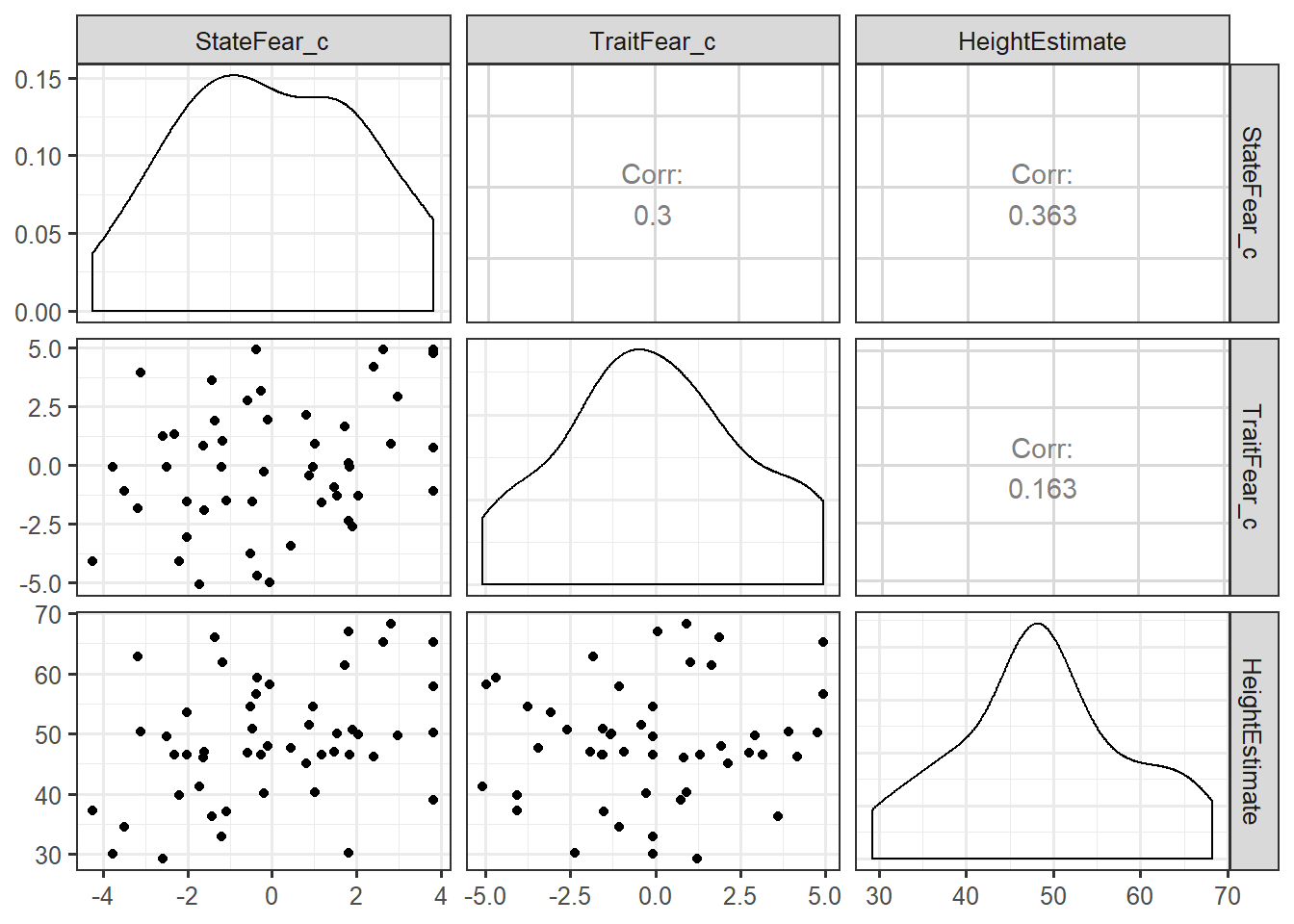
As you can see, we can now see our X1 (mean-centered state fear) and X2 (mean-centered trait fear) and X2 plotted against our dependent variable of interest, Y (height estimates). Of interest to checking the assumption of linearity, we will want to “eyeball” the scatterplots and distributions to determine if we have met our assumption of linearity. The check of the scatterplot also provides some insight into if there are any outliers, or extreme values in your dataset, as well as the variability in your dataset and how that variability moves together with other variables in your regression model. We can also get a sense of whether there is the possibility of multicollinearity before explicitly testing for this assumption - does it seem like X1 and X2 are highly correlated?
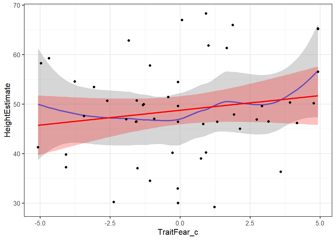
We may also want to perform a more thorough check using a loess smoother for each variable in the model. A loess smoother selectively weights points in the regression. We can also overlay the straight regression line to determine how the loess smoothing of data compares to a linear regression.
ggplot(feardata, aes(TraitFear_c,HeightEstimate)) + stat_smooth(method="loess") + stat_smooth(method="lm", color="red", fill="red", alpha=.25) + geom_point()
ggplot(feardata, aes(StateFear_c,HeightEstimate)) + stat_smooth(method="loess") + stat_smooth(method="lm", color="red", fill="red", alpha=.25) + geom_point()
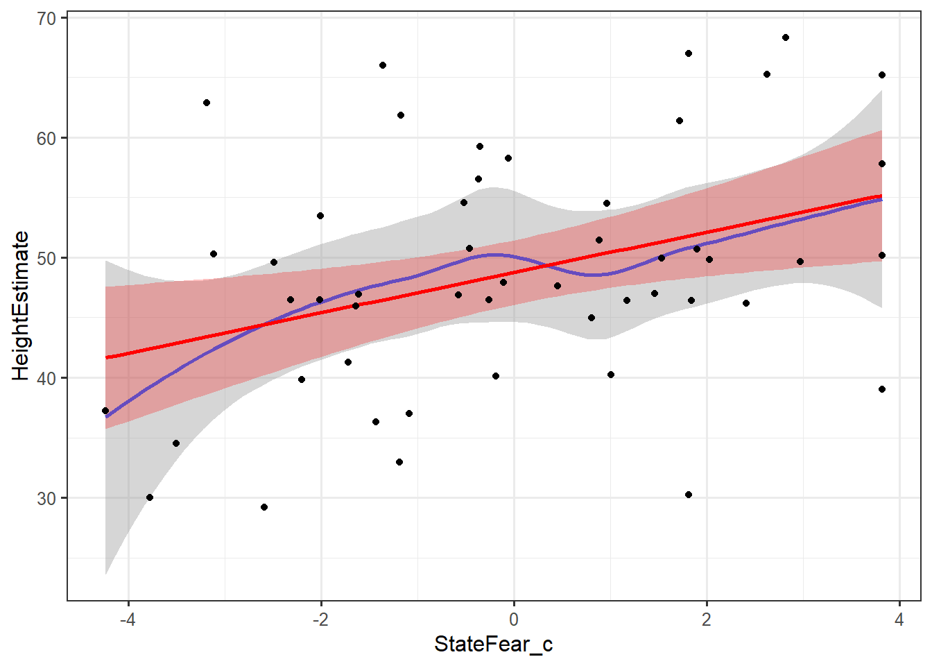
In these plots, the grey shading corresponds to the standard errors for the loess smoother fit, while the red shading corresponds to the standard errors for the linear fit. The blue line is a loess smoothed line and the red line is a linear regression line. As long as the loess smoother roughly approximates the linear line, the assumption of linearity has been met. It appears that the relationships between X’s and Y’s are roughly linear.
Checking the assumption of constant variance of residuals (Homoscedasticity)
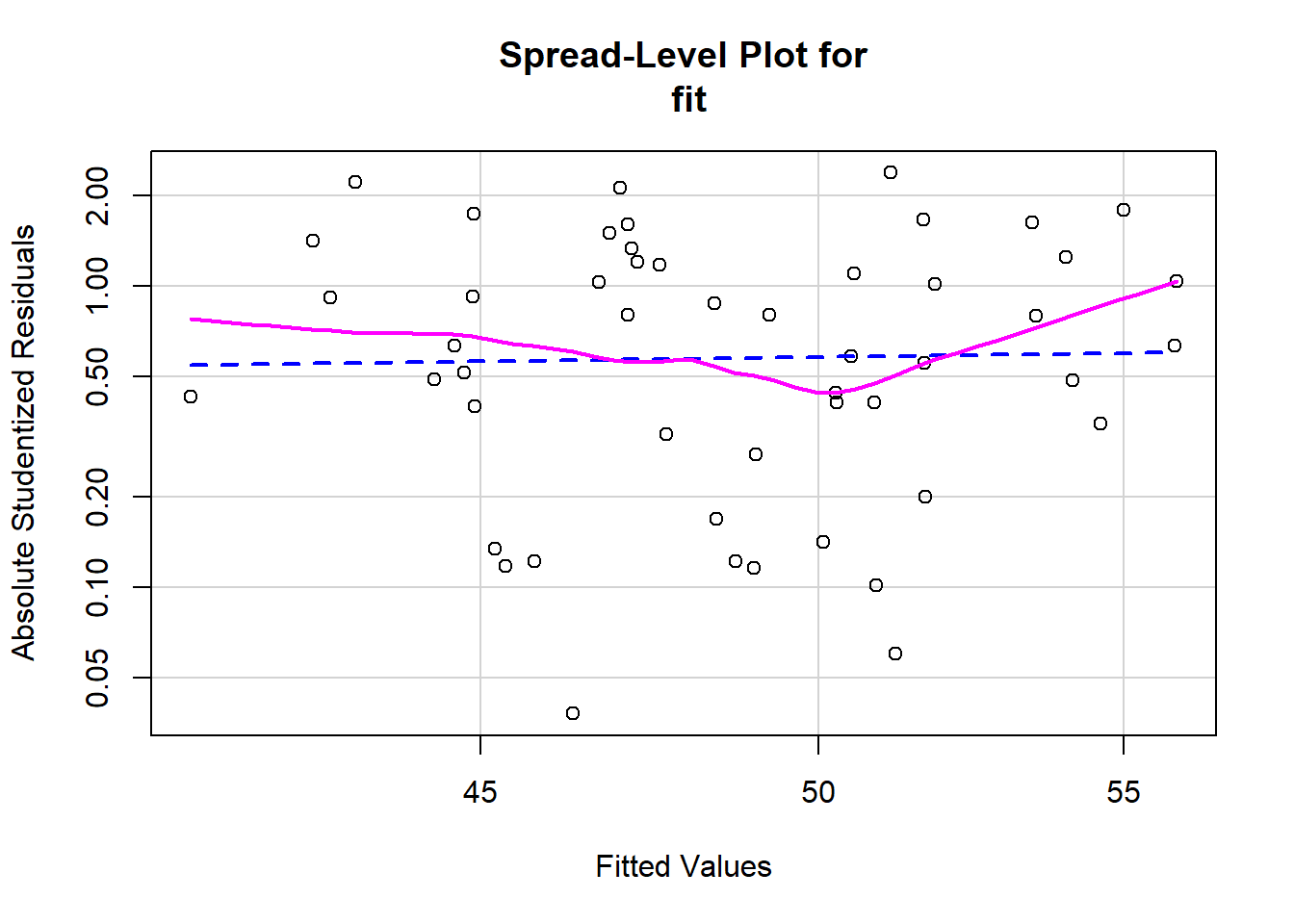
We will generate a plot with a red line (linear fit) and a dashed green line (loess smoothed fit). Again, we are looking for any lawful curves or skewness in the data that may suggest that our regression model is better or worse at predicting for specific levels of our predictors. Absolute studentized residuals refers to the absolute values (ignoring over or underfitting) of the quotient resulting from the division of a residual by an estimate of its standard deviation. These should be roughly equally distributed acros the range of the fitted Y values.
spreadLevelPlot(fit)
##
## Suggested power transformation:  0.7112184
In this case, even though there appear to possibly be some small curves in the loess smoother, the linear fit seems fairly straight across the scale. This is about on the border of homoscedastic and heteroscedastic. Whenever I’m on the border about meeting an assumption, I lean towards saying that I have met the assumption, since regression is fairly robust to minor violations of assumptions.
Checking the assumption of normality of residuals
The following code will generate a Quantile-Quantile (Q-Q) plot. Q-Q plots are used to assess whether your distibution of residuals (represented on the Y axis) roughly approximate a normal distribution of residuals (represented on the X axis). The points should mostly fall on the diagonal line in the middle of the plot. If this assumption is violated, the points will fall in some sort of curve shape, such as an S, or will form two separate, variable lines.
# Normality of Residuals
# qq plot for studentized resid
qqPlot(fit, main="QQ Plot") # distribution of studentized residuals
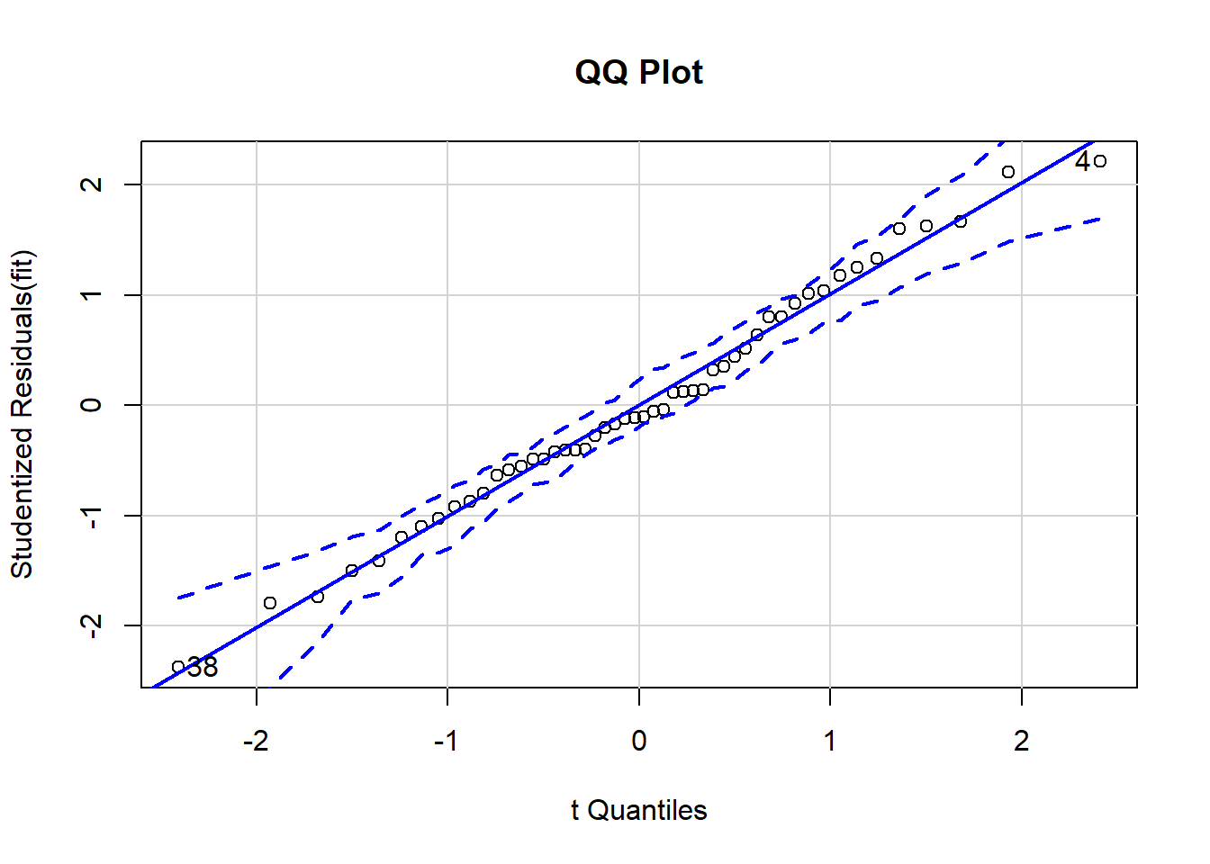
## [1] 4 38
In this example, we can see the that each observation roughly falls on the straight line, indicating that our residuals are roughly normally distributed. Though there is a little bit of bend, there is no significant curve or break in the data, so we have met this assumption. In addition, none of the points falls outside the 95% confidence intervals (depicted using the dashed lines), indicating that there are seemingly no extreme residual values (perhaps one in there, but I’m not too concerned about that). We have met the assumption of normality of residuals.
Secondly, we can also observe the histogram generated to get a 2nd perspective on whether or not the residuals are roughly normally distributed.
#Use MASS package to generate histogram of residual distribution
sresid <- studres(fit)
hist(sresid, freq=FALSE,
   main="Distribution of Studentized Residuals")
xfit<-seq(min(sresid),max(sresid),length=40)
yfit<-dnorm(xfit)
lines(xfit, yfit)
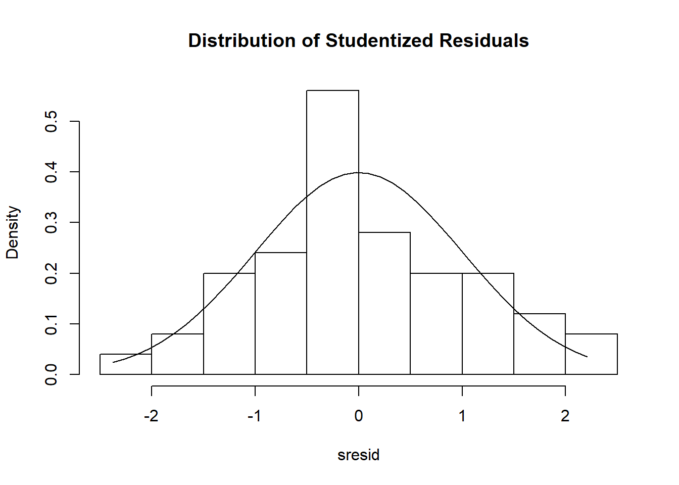 In this instance, we overlay a normal distribution curve on top of the histogram, and observe that the histogram roughly approximates a normal distribution.
Checking for multicollinearity
One of the primary indicators of multicollinearity is the variance inflation factor (VIF). The VIF indicates the amount of increase in variance of regression coefficient relative to when all predictors are uncorrelated. If the VIF of a variable is high, it means the variance explained by that variable is already explained by other X variables present in the given model, which means that variable is likely redundant. The lower the VIF, the better. If the VIF is less than 2, we meet the assumption of no multicollinearity. Note that this is a very conservative cutoff, some have recommended 10 as a reasonable cutoff. The VIF is equal to 1 divided by 1 minus R-squared.
vif(fit) # variance inflation factors
## StateFear_c TraitFear_c
##    1.098924    1.098924
sqrt(vif(fit)) > 2 #checks if the VIF's in your model are > 2, usually indicating a problem if TRUE
## StateFear_c TraitFear_c
##       FALSE       FALSE
It appears that the VIF for both of our predictors is less than 2, so we have met the assumption of multicollinearity for this model. If there is multicollinearity present in your model and you violate this assumption, however, you have the options of a) combining highly correlated predictors into a single index, b) removing (a) predictor(s), or c) using ridge regression (see McDonald, 2009, use lm.ridge function in the MASS package) and/or principal components regression (see Massey, 1965, use the pls package).
Checking the data for outliers
Lastly, once we are sure that our regression model meets all other assumptions, it is prudent to check for outlier (extreme) cases which may bias the estimation of our signifiance terms, such as p-values and 95% confidence intervals. If values are extreme enough, it is possible that a single case may change a result from “significant” to “non-significant”, and vice-versa, dependent on your chosen alpha level. If, from your initial inspection of scatterplots it appears that a few extreme cases may be causing a relationship between variables to look non-linear, it may make sense to check for and remove outliers prior to checking other assumptions.
There are three primary indicators of outlier cases. I’ll walk through each one by one.
- Leverage: How unusual is the observation in terms of its values on the independent predictors?
This first bit of code calculates leverage values (capped at 1), appends these to our dataframe, then creates leverage plots for each of our independent predictors, state fear and trait fear. Note: Make sure you keep case numbers consistent. Since we did not sort our original dataframe by student, its better to use the X column, which corresponds to row number in the data. This will make sure we know which cases (row numbers) to keep an eye on throughout outlier checks, rather than getting confused with the student (or what might be participant number) variables. If you want to use participant ID’s or similar variables, make sure to sort your dataframe by that variable before walking through each index plot.
feardata$leverage <- hatvalues(fit)
ggplot(feardata, aes(X, leverage)) + geom_point() + ylim(0,1) + xlab('Case')
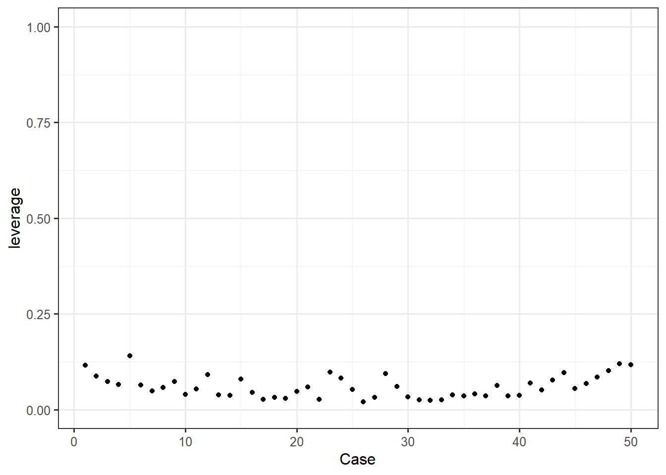 Again, we are looking for any point that visually sticks out. In this case, it doesn’t appear that any points exhibit abnormally high leverage.
If you aren’t sure about outliers from your plot or would like a more objective measure of leverage using suggested cutoffs, you can directly test whether influence measures for each observation in your model.
# list the observations with large hat value
fit.hat <- hatvalues(fit)
id.fit.hat <- which(fit.hat > (2*(4+1)/nrow(feardata))) ##  hatvalue > #2*(k+1)/n
fit.hat[id.fit.hat]
## named numeric(0)
In this case, we see that there are no extreme values listed in our dataset, at least indicated by leverage.
- Discrepancy: Amount of difference between observed and predicted values. Main indicator is called externally studentized residual. These are residuals calculated after removing each case & rerunning the regression.
Similarly for discrepancy, we can use the MASS package to generate studentized residuals (our measure of discrepancy), append these to our dataset by case, and then plot those by case. This is usually called an “index” plot where index refers to each measurement in our dataset. Studentized residuals are calculated by taking the difference between observed and predicted value and dividing by the standard error.
feardata$studres <- studres(fit) #adds the studendized residuals to our dataframe
ggplot(feardata, aes(X,studres)) + geom_point() + geom_hline(color="red", yintercept=0) + xlab('Case')
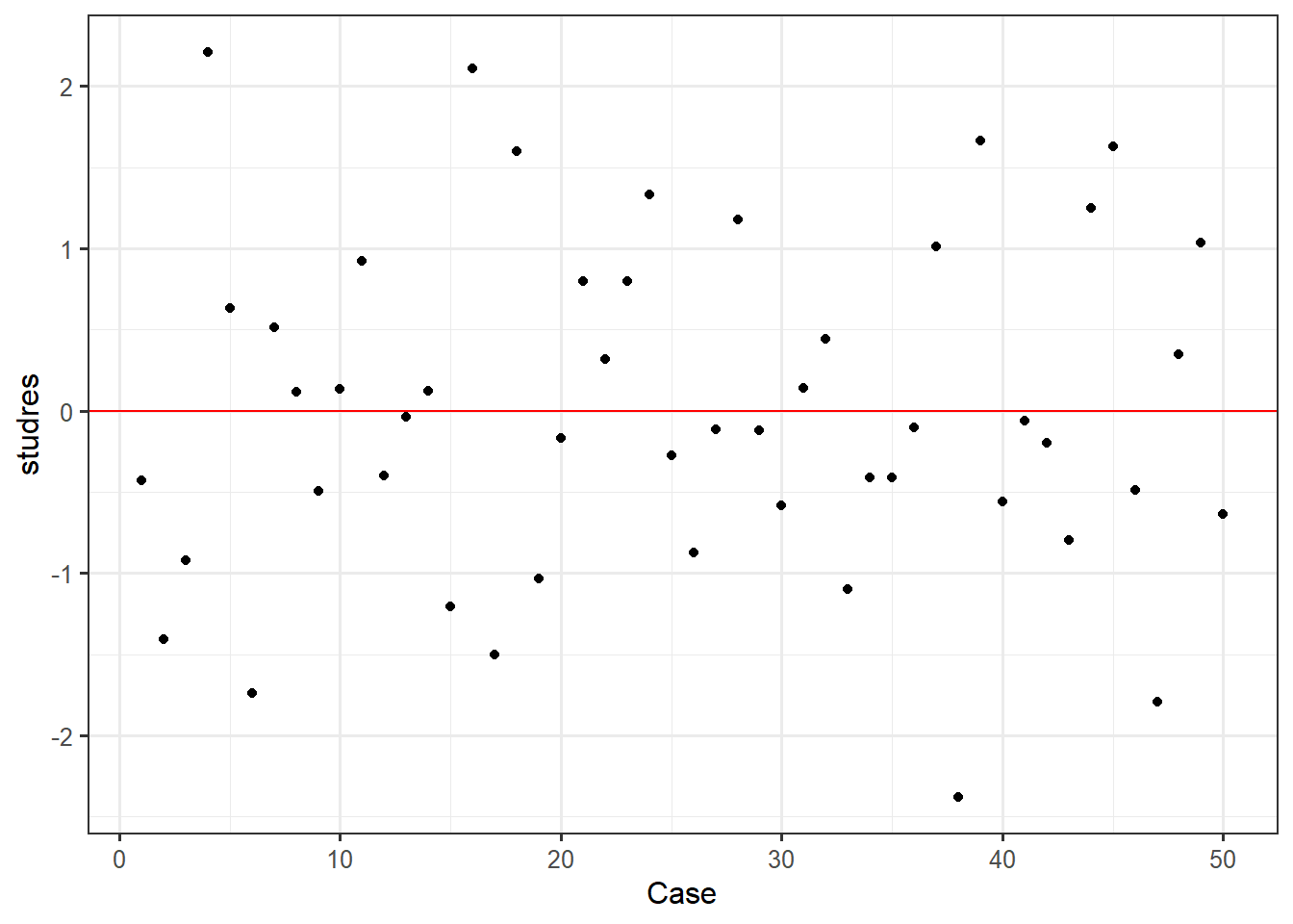 Discrepancy indicates the amount of difference between observed and predicted values. We would be looking to see if any value appears to be vastly different than others (e.g. a positive or negative 4 when the most extreme discrepancies appear to be around positive or negative 2). In this case, it doesn’t appear that any cases display extreme discrepancy.
- Influence: A combination of leverage and discrepancy. Global indicators of influence include Difference in fits, standardized (DFFITS) & Cook’s distance, and indicate how much Yhat (predicted Y) changes based on removal of a case. Specific indicators of influence (Difference in fits of betasindicate how much specific regression coefficients in your model would change
Here, we create a plot of one indicator of influence, Cook’s distance. Bollen & Jackman (1990) have defined a Cook’s distance of 4 divided by the degrees of freedom of the model as a reasonable cutoff point for extreme influence, which we will use here. Another rule-of-thumb is using k/n as the cutoff (k is # of predictors, n is sample size). This plot will provide a visual representation of which cases are most extreme in our dataset. If you want to make this look like the other plots using ggplot2, feel free, I just like this version for its ability to mark potential outliers in the plot using cutoffs.
#identify D values > 4/(n-k-1)
cutoff <- 4/((nrow(feardata)-length(fit$coefficients)-2))
plot(fit, which=4, cook.levels=cutoff)
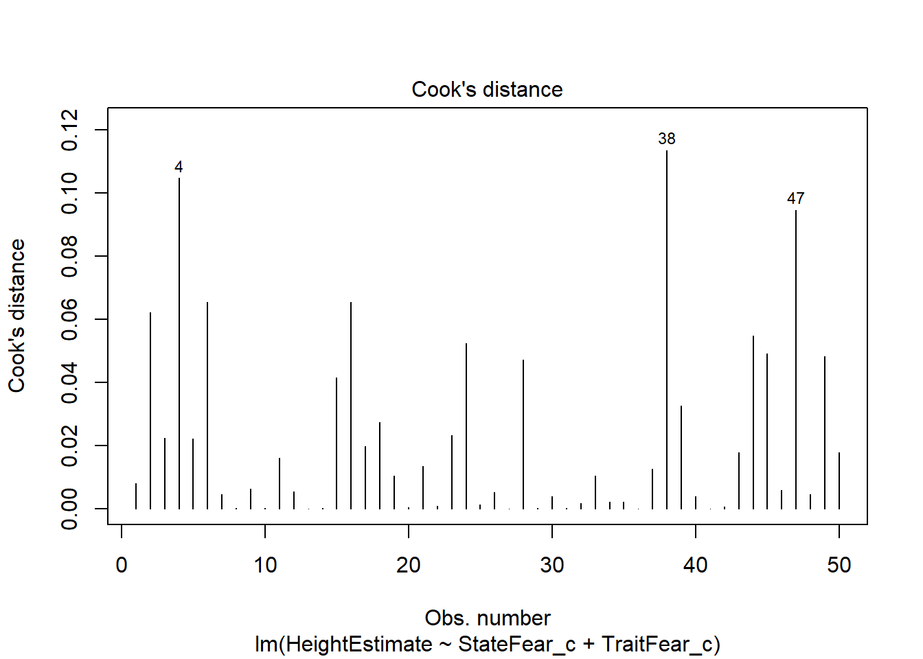
This plot marks some potentially concerning cases based on the suggested cutoff for Cook’s distance. This is likely a conservative cutoff so I’m fine with leaving these values in, though I want to check further indicators of influence to be sure.
Second, we will take a look at our DFFITS. Though these should be very similar to Cook’s distance, its good to be thorough and check multiple indicators of global influence.
feardata$dffits <- dffits(fit)
ggplot(feardata, aes(X,dffits)) + geom_point() + geom_hline(color="red", yintercept=0) + xlab('Case') + ylim(-5,5)
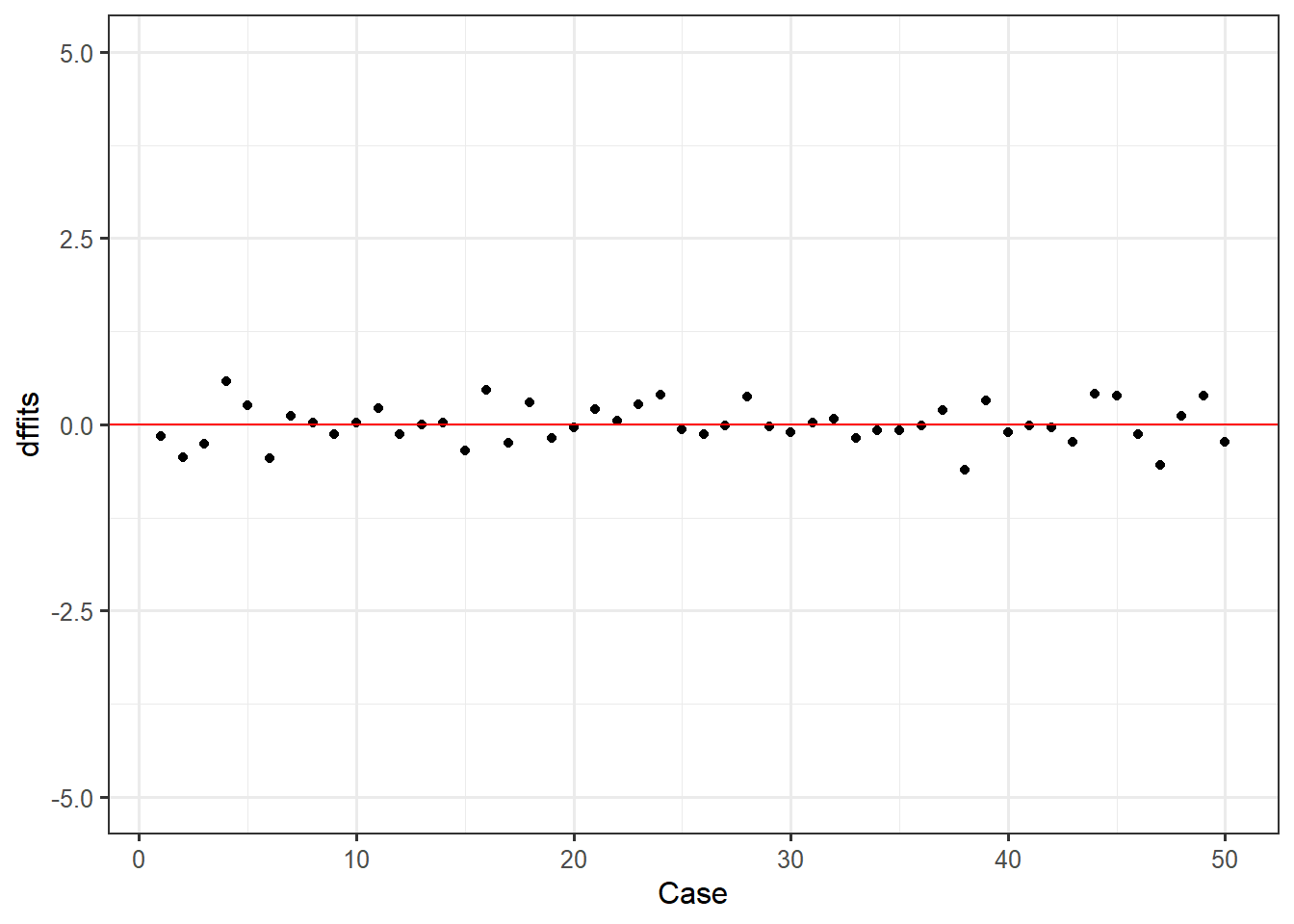 Here based on a quick look we see that no points appear to have a huge differential influence.
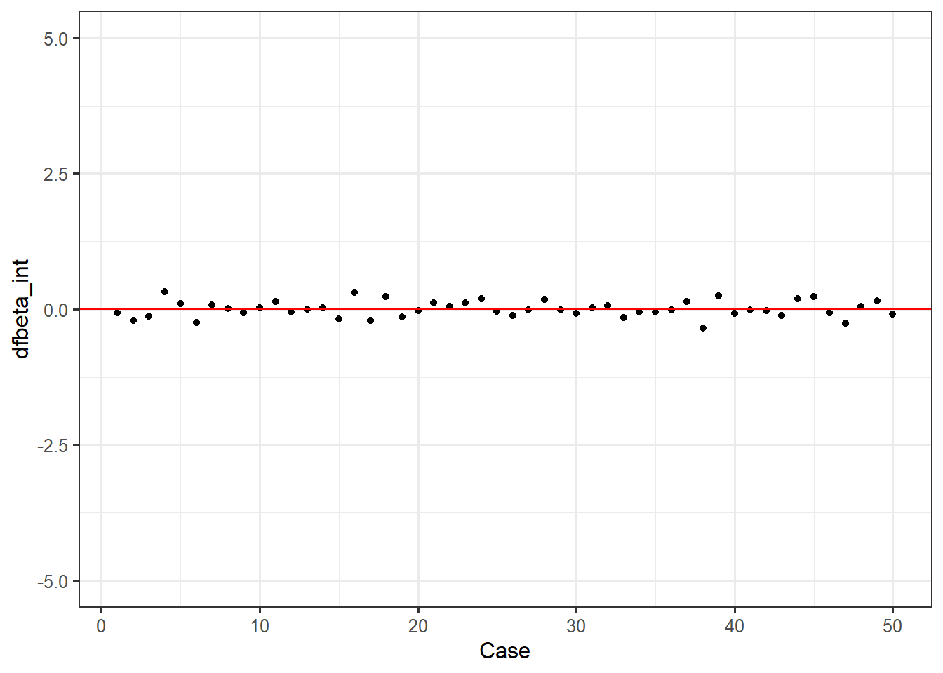
DFBetas are indicators of specific influence - how much do the regression coefficients of a single predictor change based on a single case? Again, we can take our append to dataframe approach, then make an index plot for our intercept dfbetas, state fear dfbetas, and trait fear dfbetas.
dfbetas <- dfbetas(fit)
feardata$dfbeta_int <- dfbetas[,1]
feardata$dfbeta_statefear <- dfbetas[,2]
feardata$dfbeta_traitfear <- dfbetas[,3]
ggplot(feardata, aes(X,dfbeta_int)) + geom_point() + geom_hline(color="red", yintercept=0) + xlab('Case') + ylim(-5,5)
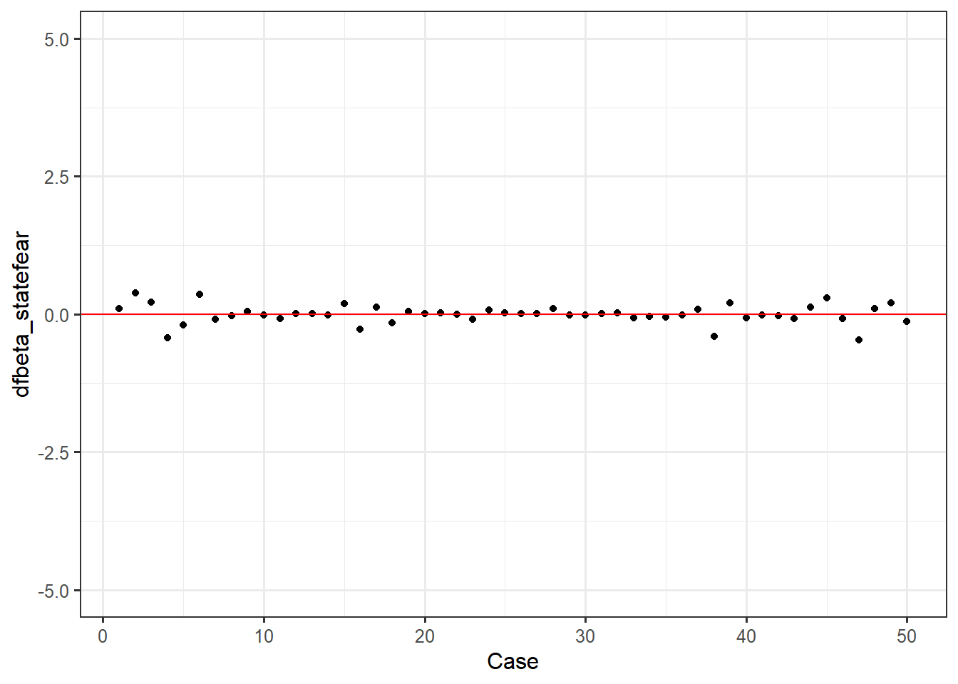
ggplot(feardata, aes(X,dfbeta_statefear)) + geom_point() + geom_hline(color="red", yintercept=0) + xlab('Case') + ylim(-5,5)
ggplot(feardata, aes(X,dfbeta_traitfear)) + geom_point() + geom_hline(color="red", yintercept=0) + xlab('Case') + ylim(-5,5)
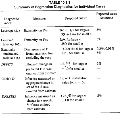
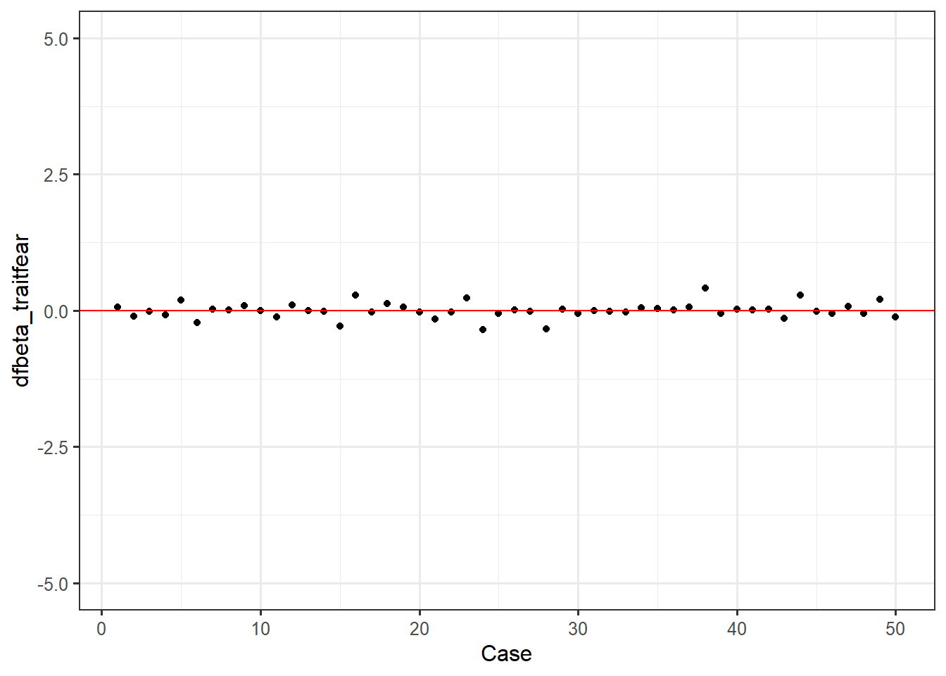 It again appears that there are no extreme values. You may be wondering: how do I make these judgment calls? Cohen, Cohen, West & Aiken (2003) nicely provide a table of suggested cutoff values for measures of leverage, discrepancy, and influence.
If plots are not your cup of tea or you want to work with numbers directly so that you can test cutoffs, use the influence.measures() function. Obviously this becomes fairly unwieldy with very large datasets, but can be a nice quick eyeball test of whether any extreme values stick out to you based on multiple indicators of influence.
influence.measures(fit)
## Influence measures of
## 	 lm(formula = HeightEstimate ~ StateFear_c + TraitFear_c, data = feardata) :
##
##      dfb.1_ dfb.StF_ dfb.TrF_    dffit cov.r   cook.d    hat inf
## 1  -0.06431  0.10257  0.06158 -0.15501 1.193 8.15e-03 0.1162   *
## 2  -0.20865  0.38309 -0.10949 -0.43626 1.030 6.21e-02 0.0874
## 3  -0.13494  0.21384 -0.01306 -0.25847 1.090 2.23e-02 0.0734
## 4   0.32319 -0.43405 -0.07781  0.58345 0.843 1.05e-01 0.0652
## 5   0.09693 -0.19158  0.19162  0.25665 1.209 2.22e-02 0.1402   *
## 6  -0.25377  0.35680 -0.21765 -0.45293 0.942 6.56e-02 0.0637
## 7   0.07453 -0.08994  0.02504  0.11683 1.103 4.62e-03 0.0491
## 8   0.01712 -0.02201  0.01462  0.02912 1.131 2.89e-04 0.0579
## 9  -0.07215  0.04344  0.09059 -0.13745 1.132 6.40e-03 0.0726
## 10  0.01939 -0.01554 -0.00595  0.02723 1.109 2.52e-04 0.0394
## 11  0.13389 -0.08315 -0.12014  0.21903 1.067 1.60e-02 0.0535
## 12 -0.05899  0.01463  0.10112 -0.12620 1.162 5.41e-03 0.0915
## 13 -0.00548  0.00491 -0.00307 -0.00755 1.109 1.94e-05 0.0379
## 14  0.01749 -0.00985 -0.00891  0.02361 1.106 1.90e-04 0.0365
## 15 -0.17742  0.19786 -0.28427 -0.35526 1.057 4.17e-02 0.0802
## 16  0.30553 -0.26905  0.28339  0.45921 0.846 6.55e-02 0.0452
## 17 -0.21490  0.12231 -0.03082 -0.24734 0.950 1.99e-02 0.0265
## 18  0.22955 -0.15833  0.13018  0.29202 0.938 2.75e-02 0.0324
## 19 -0.14808  0.05233  0.06369 -0.17774 1.025 1.05e-02 0.0288
## 20 -0.02433  0.01459 -0.02791 -0.03760 1.118 4.81e-04 0.0477
## 21  0.11690  0.02150 -0.16142  0.20130 1.088 1.36e-02 0.0593
## 22  0.04603 -0.00200 -0.02452  0.05306 1.088 9.57e-04 0.0266
## 23  0.11939 -0.08960  0.23419  0.26364 1.134 2.33e-02 0.0975
## 24  0.19687  0.07357 -0.34703  0.40026 1.038 5.25e-02 0.0827
## 25 -0.04011  0.01975 -0.05064 -0.06478 1.120 1.43e-03 0.0522
## 26 -0.12477  0.00739  0.00964 -0.12561 1.036 5.29e-03 0.0203
## 27 -0.01667  0.00458 -0.01269 -0.02097 1.101 1.50e-04 0.0316
## 28  0.17493  0.09599 -0.33503  0.37798 1.076 4.72e-02 0.0934
## 29 -0.01771 -0.01099  0.02470 -0.03062 1.133 3.19e-04 0.0598
## 30 -0.08415 -0.01219 -0.05993 -0.10804 1.079 3.95e-03 0.0330
## 31  0.02028  0.00975 -0.00595  0.02272 1.093 1.76e-04 0.0251
## 32  0.06336  0.03025 -0.01073  0.07023 1.080 1.67e-03 0.0246
## 33 -0.15768 -0.06075 -0.03324 -0.17738 1.012 1.04e-02 0.0253
## 34 -0.05898 -0.04462  0.04612 -0.08153 1.097 2.26e-03 0.0382
## 35 -0.05900 -0.04836  0.03368 -0.07889 1.094 2.11e-03 0.0358
## 36 -0.01464 -0.01315  0.01065 -0.02089 1.111 1.49e-04 0.0407
## 37  0.14591  0.09419  0.05749  0.19555 1.036 1.27e-02 0.0359
## 38 -0.34705 -0.40285  0.41015 -0.61212 0.804 1.14e-01 0.0622   *
## 39  0.23994  0.21055 -0.05704  0.31928 0.928 3.27e-02 0.0354
## 40 -0.08016 -0.07282  0.02394 -0.10832 1.085 3.97e-03 0.0365
## 41 -0.00878 -0.01080  0.01129 -0.01628 1.145 9.03e-05 0.0687
## 42 -0.02901 -0.03318  0.02342 -0.04628 1.121 7.29e-04 0.0509
## 43 -0.11739 -0.08122 -0.14858 -0.23075 1.109 1.79e-02 0.0773
## 44  0.18578  0.13167  0.28309  0.40769 1.068 5.48e-02 0.0963
## 45  0.23685  0.30056 -0.01287  0.39116 0.954 4.93e-02 0.0545
## 46 -0.07128 -0.07916 -0.04977 -0.13147 1.127 5.86e-03 0.0680
## 47 -0.26525 -0.47075  0.07072 -0.54537 0.951 9.47e-02 0.0845
## 48  0.05196  0.10325 -0.05065  0.11741 1.179 4.68e-03 0.1021
## 49  0.15598  0.20120  0.21048  0.38136 1.131 4.84e-02 0.1195
## 50 -0.09556 -0.12493 -0.12340 -0.23061 1.176 1.80e-02 0.1165
In this output, the corresponding column numbers in their respective order indicate: dfbeta of the intercept, dfbeta of X1, dfbeta of x2, dffits, covariance ratio (the change in the determinant of the covariance matrix of the estimates by deleting this observation), cook’s distance, leverage, significance test marking that case as a potential outlier.
Note that this function marks cases which may show extreme influence with asterisks. It is always good to see if cases appear multiple times across plot and numeric checks. For instance, case number 38 appears here and in the earlier Cook’s distance plot, suggesting it may be an outlier. If you are unsure whether a case is an outlier or not, it would be good to perform what is typically referred to as a sensitivity analysis. A sensitivity analysis asks the question: does our take-home message from the model change when we remove a case compared to a model that includes the case? If it does, that suggests that case is abnormally affecting regression coefficients and/or significance tests and should be removed. If not, it can probably justifiably be left in the model. For instance, let’s see what removing case 38 does to our regression results.
summary(fit) #first, let's remind ourself of the results with 38 in the model
##
## Call:
## lm(formula = HeightEstimate ~ StateFear_c + TraitFear_c, data = feardata)
##
## Residuals:
##     Min      1Q  Median      3Q     Max
## -20.931  -5.455  -1.029   6.882  19.576
##
## Coefficients:
##             Estimate Std. Error t value Pr(>|t|)
## (Intercept)  48.7580     1.3484  36.161   <2e-16 ***
## StateFear_c   1.5965     0.6583   2.425   0.0192 *
## TraitFear_c   0.2177     0.5223   0.417   0.6787
## ---
## Signif. codes:  0 '***' 0.001 '**' 0.01 '*' 0.05 '.' 0.1 ' ' 1
##
## Residual standard error: 9.534 on 47 degrees of freedom
## Multiple R-squared:  0.1348,	Adjusted R-squared:  0.09795
## F-statistic:  3.66 on 2 and 47 DF,  p-value: 0.03331
feardata.no38 <- feardata[-38,] #remove case 38 from the dataframe and assign this to a new dataframe
fit.no38 <- lm(HeightEstimate ~ StateFear_c + TraitFear_c, feardata.no38) #new model without 38
summary(fit.no38) #did our results change?
##
## Call:
## lm(formula = HeightEstimate ~ StateFear_c + TraitFear_c, data = feardata.no38)
##
## Residuals:
##     Min      1Q  Median      3Q     Max
## -17.254  -5.737  -1.319   6.798  19.563
##
## Coefficients:
##             Estimate Std. Error t value Pr(>|t|)
## (Intercept) 49.20436    1.29991  37.852  < 2e-16 ***
## StateFear_c  1.84949    0.63696   2.904  0.00565 **
## TraitFear_c  0.01335    0.50564   0.026  0.97906
## ---
## Signif. codes:  0 '***' 0.001 '**' 0.01 '*' 0.05 '.' 0.1 ' ' 1
##
## Residual standard error: 9.095 on 46 degrees of freedom
## Multiple R-squared:  0.1704,	Adjusted R-squared:  0.1343
## F-statistic: 4.724 on 2 and 46 DF,  p-value: 0.01362
We can see that though removal of this case had a decent impact on regression coefficients and p-values, none of these changes altered our take home message. We still see that state fear significantly positively predicts height estimates when controlling for trait fear, while trait fear does not significantly predict height estimates when controlling for state fear. However, perhaps inclusion of this case caused us to be conservative with our estimate of the magnitude of influence of state fear on height estimates.
Quickly and effortlessly checking many assumptions at once
If the above seems unwieldy, you’re under a time-crunch for a project deadline, or you have a good sense that you’ve met most of the assumptions already, you may want to use just a few quick functions to see if you’ve met some of the assumptions of regression. The first uses the plot function from base R, which handles lm objects differently than dataframes.
plot(fit)
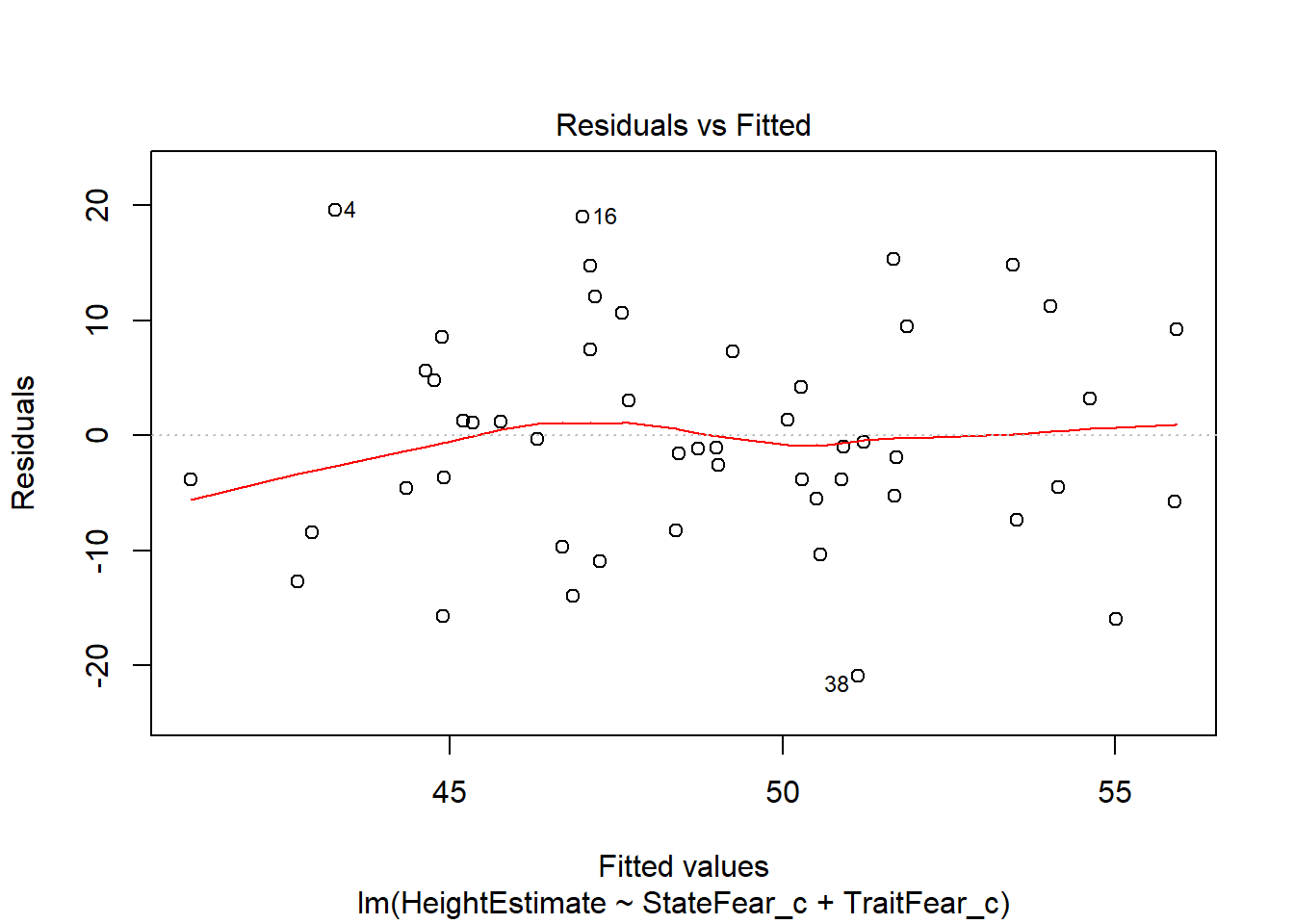
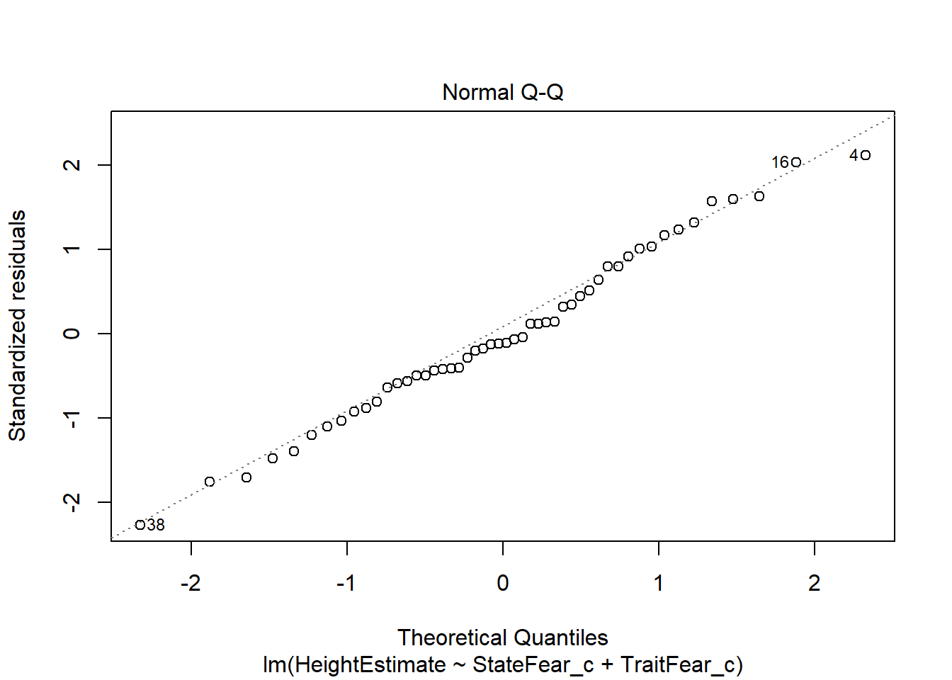
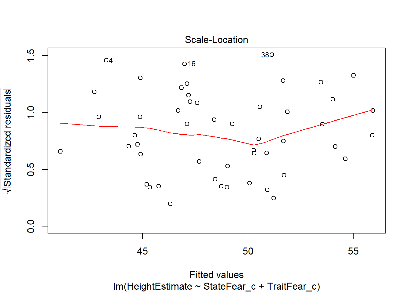
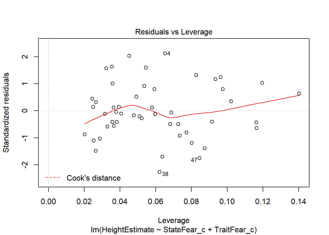 This output provides you four useful plots:
Residuals vs Fitted Values, to check constant variance in residuals and linearity of association between predictors and outcome (look for a relatively straight line and random-looking scatterplot).
Normal Q-Q Plot, to check the assumption of normally distributed residuals.
Root of Standardized residuals vs Fitted values, this is very similar to number 1, where the Y axis of residuals is in a different metric (notice cases 4, 18, and 38 are labelled again, just like our first figure).
Residuals vs Leverage, to check if the leverage of certain observations are driving abnormal residual distributions, thus violating assumptions and biasing statistical tests. Potentially problematic points will be labelled in the plot.
A second useful function is provided by the gvlma function in the gvlma package which will quickly check 5 assumptions for you.
library(gvlma)
gvlma(fit)
##
## Call:
## lm(formula = HeightEstimate ~ StateFear_c + TraitFear_c, data = feardata)
##
## Coefficients:
## (Intercept)  StateFear_c  TraitFear_c
##     48.7580       1.5965       0.2177
##
##
## ASSESSMENT OF THE LINEAR MODEL ASSUMPTIONS
## USING THE GLOBAL TEST ON 4 DEGREES-OF-FREEDOM:
## Level of Significance =  0.05
##
## Call:
##  gvlma(x = fit)
##
##                      Value p-value                Decision
## Global Stat        0.70351  0.9509 Assumptions acceptable.
## Skewness           0.11302  0.7367 Assumptions acceptable.
## Kurtosis           0.37881  0.5382 Assumptions acceptable.
## Link Function      0.17365  0.6769 Assumptions acceptable.
## Heteroscedasticity 0.03803  0.8454 Assumptions acceptable.
These assumptions are:
Are the relationships between your X predictors and Y roughly linear? Rejection of the null (p < .05) indicates a non-linear relationship between one or more of your X’s and Y. This means that you should likely use an alternative modeling technique or add an additional transformed X term to your model to agree with the data structure (e.g. add a quadratic term, X-squared, to the model if the relationship seems curvilinear from further scatterplot inspection).
Is your distribution skewed positively or negatively, necessitating a transformation to meet the assumption of normality? Rejection of the null (p < .05) indicates that you should likely transform your data.
Is your distribution kurtotic (highly peaked or very shallowly peaked), necessitating a transformation to meet the assumption of normality? Rejection of the null (p < .05) indicates that you should likely transform your data.
Is your dependent variable truly continuous, or categorical? Rejection of the null (p < .05) indicates that you should use an alternative form of the generalized linear model (e.g. logistic or binomial regression).
Is the variance of your model residuals constant across the range of X (assumption of homoscedastiity)? Rejection of the null (p < .05) indicates that your residuals are heteroscedastic, and thus non-constant across the range of X. Your model is better/worse at predicting for certain ranges of your X scales.
I would encourage you to thoroughly check the assumptions as I laid out previously rather than doing any of the quick tests suggested in the last portion of the tutorial. The earlier checks are more thorough and allow you more fine-grained insight into the nature of your dataset and model. However, the last suggestions are usually a good first pass at knowing if one or more assumptions may be violated in your model.
Thank you for reading! I hope this helped you bridge the gap between regression-based concepts and doing regression in R. Remember that these steps should always be taken prior to analysis so that you can interpret and report your model results with confidence. For additional documentation, please reference Cohen, Cohen, West, and Aiken (2003, Chp 4 & Chp 6). Note that asssumptions are slightly different for multilevel regression models (for nested data structures, such as trials within individuals, or individuals within schools) and other forms of the generalized linear model. I hope to make a tutorial for checking the assumptions of alternative regression approaches soon. Please email me at Ian.Ruginski@utah.edu if you have any questions or suggestions.
References
Bollen, Kenneth A.; Jackman, Robert W. (1990). Fox, John; Long, J. Scott, eds. Regression Diagnostics: An Expository Treatment of Outliers and Influential Cases. Modern Methods of Data Analysis. Newbury Park, CA: Sage. pp. 257-291.
Cohen, J., Cohen, J., Cohen, P., West, S. G. A., Leona, S., Patricia Cohen, S. G. W., & Leona, S. A. (2003). Applied multiple regression/correlation analysis for the behavioral sciences.
Massy, W. F. (1965). Principal components regression in exploratory statistical research. Journal of the American Statistical Association, 60(309), 234-256.
McDonald, G. C. (2009). Ridge regression. Wiley Interdisciplinary Reviews: Computational Statistics, 1(1), 93-100.
Raudenbush, S. W., & Bryk, A. S. (2002). Hierarchical linear models: Applications and data analysis methods (Vol. 1). Sage. Chicago.
© 2016 Ian Ruginski. Built using RMarkdown; Licensed under the Creative Commons License.
Ian Ruginski
Postdoctoral Fellow
My research interests include spatial cognition, navigation, data visualization, and human-computer interaction.