Structural Equation Modeling in R Tutorial 1: Two predictor regression using R
Table of Contents
Made for Jonathan Butner’s Structural Equation Modeling (SEM) Class, Fall 2017, University of Utah. This handout begins by showing how to import data into R. Then, correlation matrices are generated, followed by a two predictor regression analysis. Lastly, it is shown how to output a matrix as an external file and use it for regression. This syntax imports the 52 cases from datafile Grade230.txt.
Data Input and Cleaning
First, we’ll load required packages.
## this calls the packages required. use
## install.packages('packagename') if not installed.

library(dplyr)  #for cleaning data
library(car)  #for scatterplotting
library(Hmisc)  #for significance of correlation coefficients
library(psych)  #for doing regression from a correlation matrix, getting descriptives
library(scatterplot3d)  #for making 3d scatterplots
library(MASS)  #for saving some casewise diagnostics
library(lavaan)  #doing regression from a covariance matrix, eventually we will use this for SEM
Then, we will read in datafile using Fortran and clean up the datafile a little bit.
# make sure to set your working directory to where the file
# is located, e.g. setwd('D:/Downloads/Handout 1 -
# Regression') you can do this in R Studio by going to the
# Session menu - 'Set Working Directory' - To Source File
# Location
grades <- read.fortran("GRADE230.txt", c("F3.0", "F5.0", "F24.0",
    "7F2.0", "F3.0", "2F2.0", "F4.0", "4F2.0", "F4.0"))
# note: #The format for a field is of one of the following
# forms: rFl.d, rDl.d, rXl, rAl, rIl, where l is the number
# of columns, d is the number of decimal places, and r is the
# number of repeats. F and D are numeric formats, A is
# character, I is integer, and X indicates columns to be
# skipped. The repeat code r and decimal place code d are
# always optional. The length code l is required except for X
# formats when r is present.

# add column names
names(grades) <- c("case", "sex", "T1", "PS1", "PS2", "PS3",
    "PS4", "PS5", "PS6", "PS7", "T2", "PS8", "PS9", "T3", "PS10",
    "PS11", "PS12", "PS13", "T4")

# selects a subset of the data for analysis, stores in new
# dataframe
grades.sub <- subset(grades, grades$case < 21 & grades$case !=
    9)
# != indicates does not equal

# lets take a look at the datafile
grades.sub  #note that R treats blank cells in your original data as missing, and labels these cases NA. NA is the default
##    case sex T1 PS1 PS2 PS3 PS4 PS5 PS6 PS7 T2 PS8 PS9 T3 PS10 PS11 PS12
## 1     1   2 75   2   1   4   4   3   2   3 63   4   2 76    1    2    3
## 2     2   2 96   2   3   4   3   6   4   2 85   4   4 96    4    4    4
## 3     3   1 97   4   2   4   3   6   3   4 99   4   4 98    4   NA    4
## 4     4   2 80   1   2   1   4   6   4   3 73   4   3 80    4    3    4
## 5     5   1 90   3   4   4   4   6   4   4 91   4   4 93    4    4    4
## 6     6   2 84   2   4   3   4   6   4   4 81   1   3 77    4    4    4
## 7     7   1 80   4   1   2   3   6   4   4 78   4   4 88    4    3    3
## 8     8   2 90   1   2   4   4   6   4   3 85   4   4 87    1    4    4
## 10   10   2 89   4   3   3   4   6   4   4 90   4   4 89    4    4    4
## 11   11   2 63   1   3   1   1   2   4   2 58   3   4 66   NA    4    3
## 12   12   1 94   2   2   4   4   6   4   2 75   2   4 89    3    3    4
## 13   13   2 91   1   4   3   3   6   3   3 97   4   4 98    3    3    4
## 14   14   1 86   3   3   2   4   6   4   4 78   1   3 85    4    4    4
## 15   15   2 97   3   4   4   4   6   4   4 86   4   4 87    4    4    4
## 16   16   1 80   1   1   4   3   6   4   1 66   2  NA 75   NA   NA   NA
## 17   17   2 82   4   4   3   4   6   4   4 86   4   2 91    4    3    4
## 18   18   2 90   4   4   4   4   6   4   4 88   4   4 99    4    4    4
## 19   19   2 92   4   3   3   3   6   4   3 83   4  NA 86    3    4    4
## 20   20   2 94   3   3   2   4   6   4   1 83   4   4 94    3    4    4
##    PS13  T4
## 1     1  62
## 2     3  94
## 3     4  96
## 4     4  55
## 5     4 103
## 6     2  86
## 7     4  68
## 8    NA  68
## 10    4  97
## 11    4  55
## 12    3 105
## 13    4 102
## 14    3  91
## 15    4  99
## 16   NA  65
## 17    4  73
## 18    4  95
## 19    4 100
## 20    4  98
# subset out specific tests using dplyr
grades.test <- dplyr::select(grades.sub, c(T1, T2, T4))


# get descriptives using psych package
describe(grades.test)
##    vars  n  mean    sd median trimmed   mad min max range  skew kurtosis
## T1    1 19 86.84  8.67     90   87.65  8.90  63  97    34 -1.00     0.59
## T2    2 19 81.32 10.79     83   81.65  7.41  58  99    41 -0.49    -0.49
## T4    3 19 84.84 17.54     94   85.41 11.86  55 105    50 -0.50    -1.48
##      se
## T1 1.99
## T2 2.47
## T4 4.02
Note that R treats blank cells in your original data as missing, and labels these cases NA. NA is the default missing data label implemented by R.
Create and Export a Correlation Matrix
Now, we’ll create a correlation matrix and show you how to export a correlation matrix to an external file on your computer harddrive. Note that the first correlation matrix created uses the option “pairwise.complete.obs”, which implements pairwiise deletion for missing data. This is usually undesirable, as it deletes variables, not entire cases, and thus can bias paramter estimates. The second option, “complete obs”, implements listwise deletion for missing data, which is more desirable than pairwise deletion because parameter estimates are less biased (entire cases are deleted, not just specific variables).
# create a correlation matrix amongst variables
grades.cor <- cor(grades.test, use = "pairwise.complete.obs",
    method = "pearson")
grades.cor  #print the correlation matrix
##           T1        T2        T4
## T1 1.0000000 0.7854925 0.8322846
## T2 0.7854925 1.0000000 0.7107027
## T4 0.8322846 0.7107027 1.0000000
rcorr(as.matrix(grades.test)) #need if you want significance of correlations, but only uses pairwise. From Hmisc pacakge.
##      T1   T2   T4
## T1 1.00 0.79 0.83
## T2 0.79 1.00 0.71
## T4 0.83 0.71 1.00
##
## n= 19
##
##
## P
##    T1     T2     T4
## T1        0.0000 0.0000
## T2 0.0000        0.0006
## T4 0.0000 0.0006
# save out the correlation matrix to a file
write.csv(grades.cor, "corroutPW.csv")
grades.cor <- cor(grades.test, use = "complete.obs", method = "pearson")
grades.cor  #notice the differences when we use listwise deletion
##           T1        T2        T4
## T1 1.0000000 0.7854925 0.8322846
## T2 0.7854925 1.0000000 0.7107027
## T4 0.8322846 0.7107027 1.0000000
# save out correlation matrix to a file on your harddrive
write.csv(grades.cor, "corroutLW.csv")
Multiple Regression
Now, we’ll do some multiple regression. Specifically we’ll ask whether tests 1 and 2 predict test 4. We’ll also check some model assumptions, including whether or not there are outliers present and whether or not there is multicollinearity amongst tests (Variance inflation factor, or VIF). Some of this code helps you to save out residuals, predicted values, and other casewise diagnostics to a dataframe for later inspection. Note that the lm command defaults to listwise deletion.
model <- lm(T4 ~ T1 + T2, data = grades.test)
# print out model results
anova(model)
## Analysis of Variance Table
##
## Response: T4
##           Df Sum Sq Mean Sq F value     Pr(>F)
## T1         1 3835.1  3835.1 37.0880 0.00001563 ***
## T2         1   46.9    46.9  0.4534     0.5103
## Residuals 16 1654.5   103.4
## ---
## Signif. codes:  0 '***' 0.001 '**' 0.01 '*' 0.05 '.' 0.1 ' ' 1
summary(model)
##
## Call:
## lm(formula = T4 ~ T1 + T2, data = grades.test)
##
## Residuals:
##     Min      1Q  Median      3Q     Max
## -22.304  -6.051   2.389   7.316  11.323
##
## Coefficients:
##             Estimate Std. Error t value Pr(>|t|)
## (Intercept) -60.5304    24.1591  -2.505  0.02341 *
## T1            1.4476     0.4468   3.240  0.00513 **
## T2            0.2418     0.3591   0.673  0.51034
## ---
## Signif. codes:  0 '***' 0.001 '**' 0.01 '*' 0.05 '.' 0.1 ' ' 1
##
## Residual standard error: 10.17 on 16 degrees of freedom
## Multiple R-squared:  0.7012,	Adjusted R-squared:  0.6638
## F-statistic: 18.77 on 2 and 16 DF,  p-value: 0.0000636
# save out fitted values and predicted values to dataframe
grades.test$Predicted <- predict(model)
grades.test$Residuals <- residuals(model)

# save out casewise diagnostics (outliers)
grades.test$leverage <- hatvalues(model)
grades.test$distance <- studres(model)
grades.test$dffits <- dffits(model)  #measure of global influence
grades.test$dfbetas <- dfbetas(model)  #measure of specific influence

# test of multicollinearity
vif(model)
##       T1       T2
## 2.610956 2.610956
# or you can use a more general command for casewise
# diagnostics:
influence.measures(model)
## Influence measures of
## 	 lm(formula = T4 ~ T1 + T2, data = grades.test) :
##
##     dfb.1_   dfb.T1    dfb.T2   dffit cov.r  cook.d    hat inf
## 1  -0.0507  0.00189  0.036633 -0.0710 1.536 0.00179 0.2130
## 2   0.1325 -0.16914  0.104782 -0.2177 1.352 0.01655 0.1492
## 3   0.2279  0.04233 -0.262393 -0.4327 1.322 0.06347 0.2039
## 4  -0.4318  0.14810  0.121694 -0.6369 0.649 0.11342 0.0906
## 5  -0.0643 -0.16422  0.294625  0.4275 1.045 0.05938 0.1143
## 6   0.0570 -0.06392  0.047855  0.1416 1.229 0.00700 0.0662
## 7  -0.1405  0.13741 -0.078404 -0.2097 1.251 0.01524 0.1014
## 8   0.1702 -0.10022 -0.057853 -0.6740 0.406 0.10982 0.0605   *
## 10 -0.0180 -0.11017  0.175121  0.2501 1.234 0.02152 0.1100
## 11  1.3245 -0.79662 -0.000893  1.3666 1.559 0.58314 0.4729   *
## 12 -0.3261  0.81391 -0.781289  0.9276 1.232 0.27151 0.3115
## 13 -0.0639 -0.23544  0.382848  0.4511 1.390 0.06928 0.2338
## 14  0.0341  0.04659 -0.074612  0.2092 1.133 0.01489 0.0609
## 15  0.0501 -0.06051  0.035416 -0.0773 1.441 0.00212 0.1632
## 16 -0.1403 -0.09122  0.223810 -0.3117 1.357 0.03356 0.1801
## 17 -0.1198  0.24069 -0.233552 -0.2984 1.367 0.03084 0.1805
## 18 -0.0232 -0.01919  0.052255  0.1135 1.273 0.00453 0.0761
## 19 -0.0955  0.13903 -0.091608  0.2271 1.193 0.01769 0.0864
## 20 -0.0472  0.06981 -0.048894  0.0924 1.372 0.00302 0.1257
model.cov <- vcov(model)  #save variance covariance matrix for cofficients
grades.cov <- cov(grades.test)  #save covariance matrix from raw data
Model results and what they mean:
Multiple R-squared tells you the porportion of variance in the dependent variable that is predicted or accounted for given the linear combination of the independent variables in your model.
Adjusted R-squared tells you an estimate of the population level R-squared value.
Residual standard error tells you the average standard deviation of the residuals (raw metric). If squared is the mean square error (MSE), included in the anova table next to residual.
Significance term following F-statistic provide an omnibus test against an intercept only model with no predictors (does your model predict your outcome better than just a mean?)
Analysis of Variance table Mean Sq the variance of the residuals
Variance inflation factor tells you whether there is multicollinearity amongst predictors in your model. Usually a number greater than 10 indicates a problem. Lower is better.
Influence measures provide a number of casewise diagnostics. In this output, the corresponding column numbers in their respective order indicate: dfbeta of the intercept, dfbeta of X1 , dfbeta of x2, dffits (global influence, or how much Yhat (predicted Y) changes based on removal of a case), covariance ratio (the change in the determinant of the covariance matrix of the estimates by deleting this observation), cook’s distance (also influence), leverage (how unusual is the observation in terms of its values on the independent predictors?), significance test marking that case as a potential outlier. Note that one way to spot outliers is to look for residuals that are more than 2 SDs beyond the mean (mean is always 0). See this webpage I made for more on checking the assumptions of regression.
Next, let’s make some plots of the models.
# making plots of the model using car package
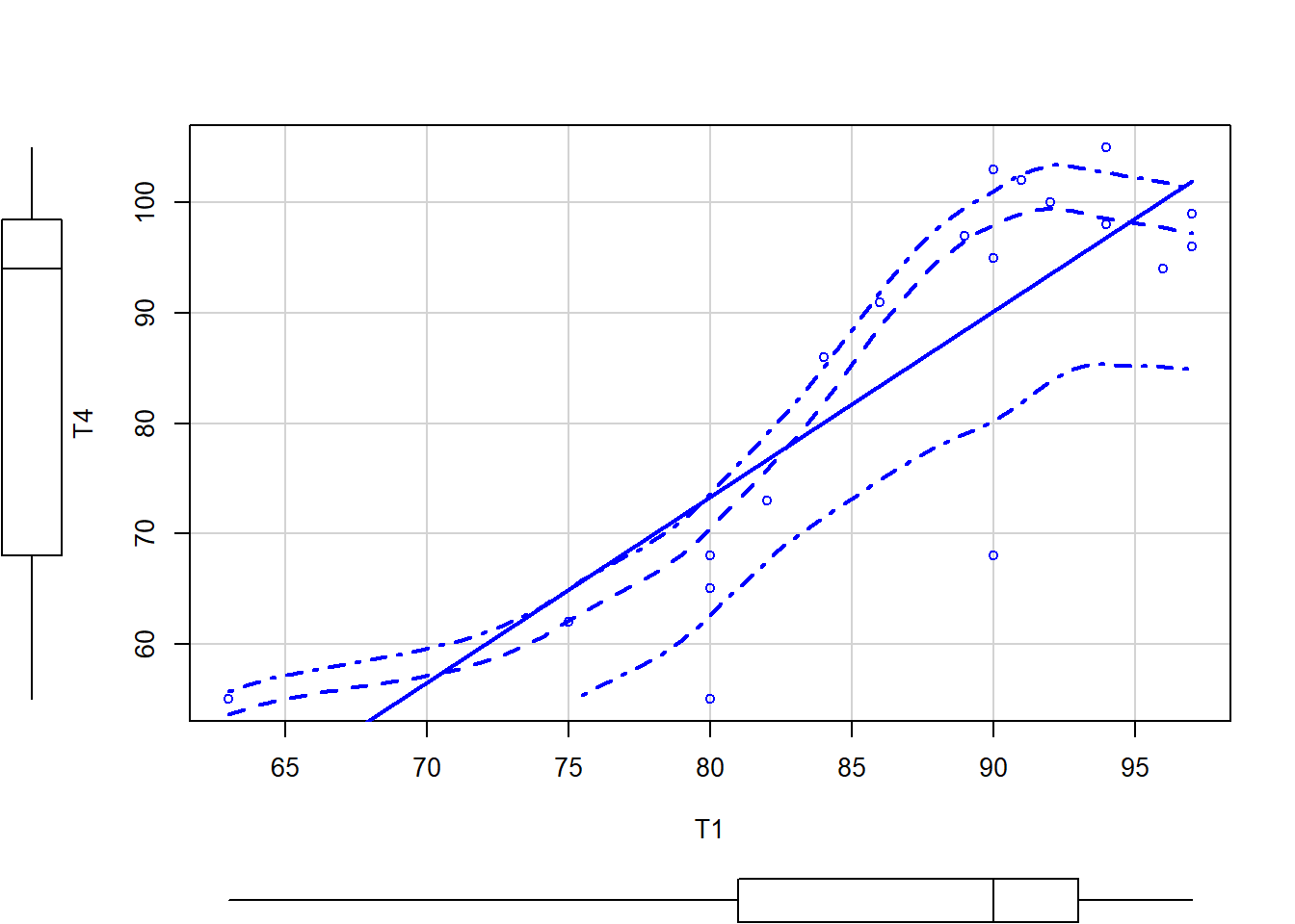
scatterplot(T4 ~ T1, data = grades.test)
scatterplot(Residuals ~ T1, data = grades.test)
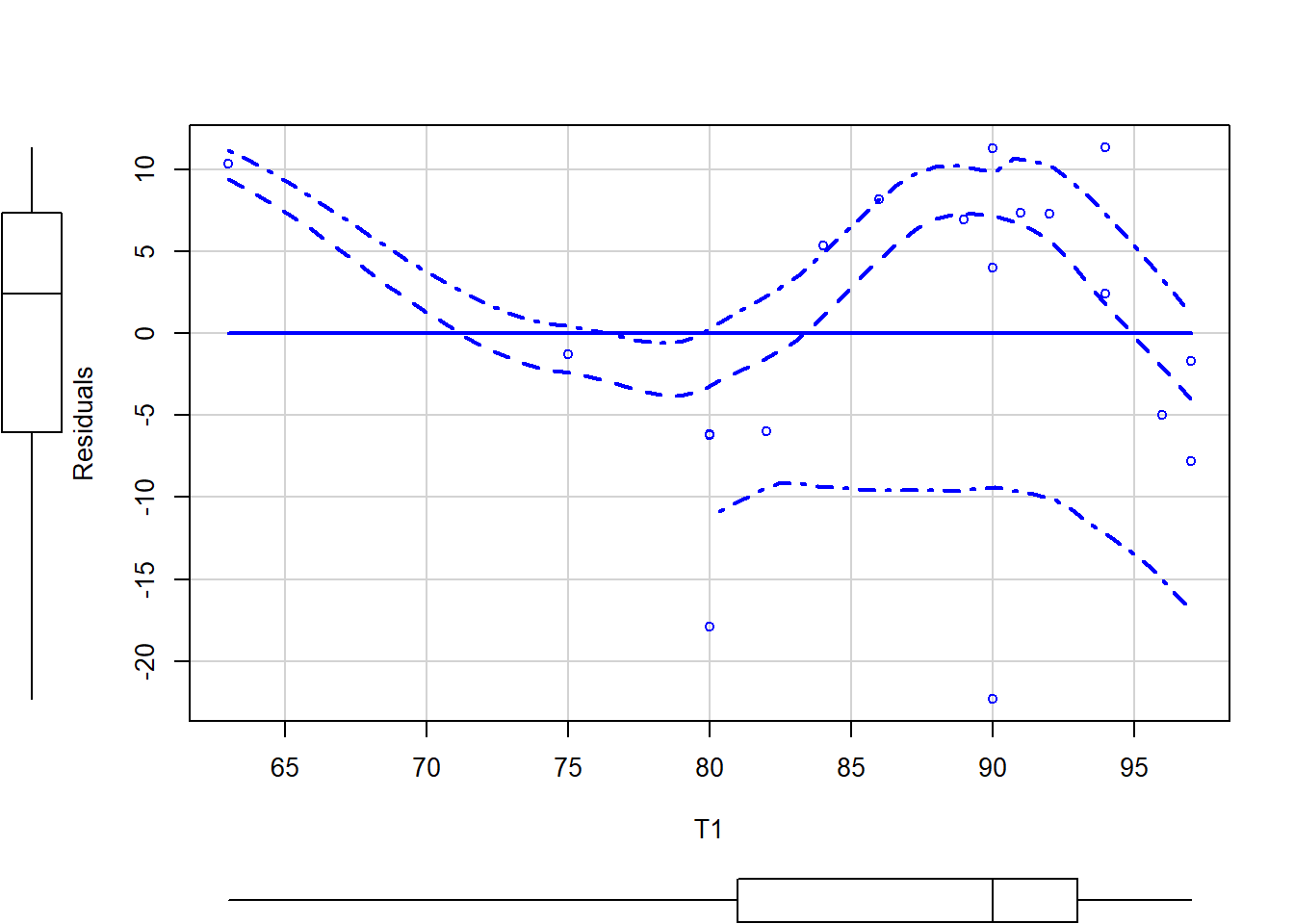 The green line indicates a linear best fit while the red line shows a loess fit. The dashed red line indicates +-1 standard error of the loess smoothed fitted line. The extra arguments to the first scatterplot command label each datapoint to help with outlier identification. Note for the second plot that, if the residuals were normally distributed, we would have a flat line rather than a curved line.
Using Multiple Regression to show how coefficients are a function of residuals
Now, lets look at how the coefficients are a function of residuals. We will build the coefficient for T1 from the previous regression. First we will create a residual of T4 (the criterion) controlling for the predictors other than T1.
model.t4 <- lm(T4 ~ T2, data = grades.test)
grades.test$model.t4resid <- residuals(model.t4)  #saves residuals to original dataframe
Next we create residuals for T1 (the predictor) controlling for the predictors other than T1. We regress T1 on T2, giving us Y=b0+b1T2 where Y is T1. What remains (the residuals, which we save out) is everything unrelated to T2.
model.t1 <- lm(T1 ~ T2, data = grades.test)
grades.test$model.t1resid <- residuals(model.t1)  #saves residuals to original dataframe
Now we run the regression using T4 with all of T2 removed as the DV and T1 with all of T2 removed as the independent variable.
model.final <- lm(model.t4resid ~ model.t1resid, data = grades.test)
anova(model.final)
## Analysis of Variance Table
##
## Response: model.t4resid
##               Df Sum Sq Mean Sq F value   Pr(>F)
## model.t1resid  1 1085.5 1085.53  11.154 0.003882 **
## Residuals     17 1654.5   97.32
## ---
## Signif. codes:  0 '***' 0.001 '**' 0.01 '*' 0.05 '.' 0.1 ' ' 1
summary(model.final) #print model results
##
## Call:
## lm(formula = model.t4resid ~ model.t1resid, data = grades.test)
##
## Residuals:
##     Min      1Q  Median      3Q     Max
## -22.304  -6.051   2.389   7.316  11.323
##
## Coefficients:
##                            Estimate            Std. Error t value Pr(>|t|)
## (Intercept)   0.0000000000000002775 2.2632510024716858688    0.00  1.00000
## model.t1resid 1.4475983535947984926 0.4334474113766849657    3.34  0.00388
##
## (Intercept)
## model.t1resid **
## ---
## Signif. codes:  0 '***' 0.001 '**' 0.01 '*' 0.05 '.' 0.1 ' ' 1
##
## Residual standard error: 9.865 on 17 degrees of freedom
## Multiple R-squared:  0.3962,	Adjusted R-squared:  0.3607
## F-statistic: 11.15 on 1 and 17 DF,  p-value: 0.003882
Note that the regression coefficient is identical to the coefficient in the two predictor regression from earlier. Next, we’re going to run another regression with the case as the DV. We will create a new graph to show that leverage is only dependent on the predictor and not the dependent variable.
model.leverage <- lm(case ~ T1 + T2, data = grades.sub)
grades.sub$leverage <- hatvalues(model.leverage)
anova(model.leverage)
## Analysis of Variance Table
##
## Response: case
##           Df Sum Sq Mean Sq F value Pr(>F)
## T1         1  12.83  12.831  0.3185 0.5804
## T2         1   5.14   5.144  0.1277 0.7255
## Residuals 16 644.66  40.291
summary(model.leverage)
##
## Call:
## lm(formula = case ~ T1 + T2, data = grades.sub)
##
## Residuals:
##     Min      1Q  Median      3Q     Max
## -9.8927 -4.7315 -0.2626  4.3500  8.2985
##
## Coefficients:
##             Estimate Std. Error t value Pr(>|t|)
## (Intercept)  1.83514   15.08035   0.122    0.905
## T1           0.17568    0.27889   0.630    0.538
## T2          -0.08009    0.22413  -0.357    0.726
##
## Residual standard error: 6.348 on 16 degrees of freedom
## Multiple R-squared:  0.02713,	Adjusted R-squared:  -0.09448
## F-statistic: 0.2231 on 2 and 16 DF,  p-value: 0.8025
scatterplot(leverage ~ case, data = grades.sub)
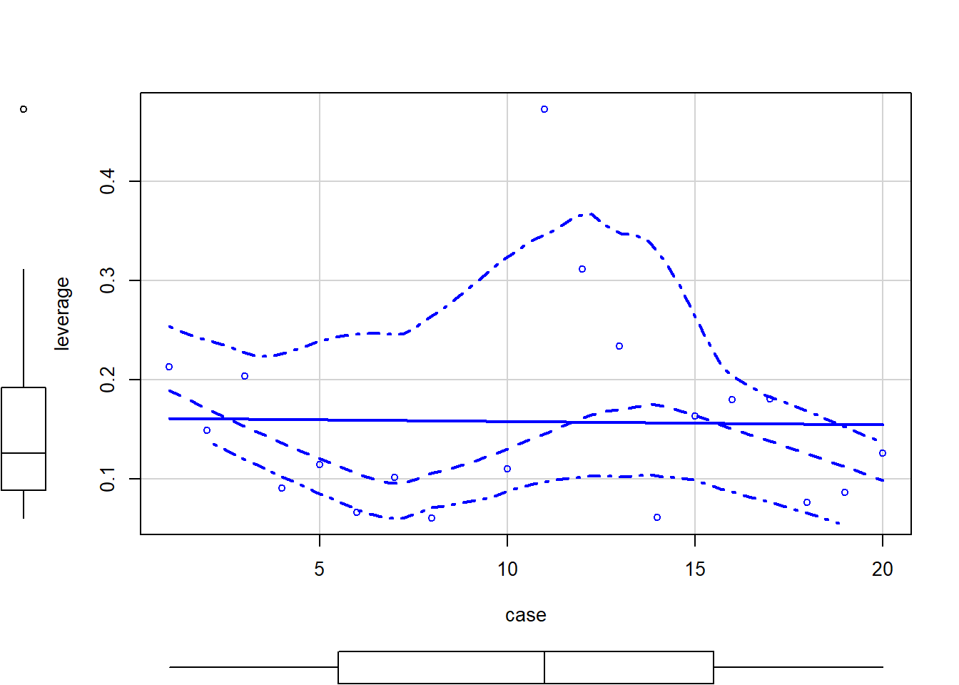
Note that in SEM there is no simple distance or leverage measures, but we can get at leverage as it is separate from the DV. If we can identify a case that is extreme we run the analyses with and without the case to determine its impact. The change in the output would be the test of leverage.
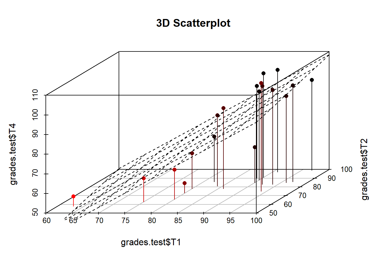
Now we will make a 3d scatterplot of relationship between tests.
s3d <- scatterplot3d(grades.test$T1, grades.test$T2, grades.test$T4,
    pch = 16, highlight.3d = TRUE, type = "h", main = "3D Scatterplot")
s3d$plane3d(model)  #uses our model from earlier to draw a regression plane
##Multiple regression using a correlation matrix
Now we will show how to do regression using just a correlation matrix. This is extremely useful if you want to do additional analyses on existing papers that provide a correlation and/or covariance matrix, but you do not have access to the raw data from those papers.
# call in correlation matrix from file on your computer.
cormatlw <- read.csv("corroutLW.csv", row.names = 1)  #tells R that first column contains row names
cormatlw <- data.matrix(cormatlw)  #change from dataframe to matrix

# do regression with the correlation matrix without raw data
model.cor <- setCor(y = "T4", x = c("T1", "T2"), data = cormatlw,
    n.obs = 18, std = FALSE)
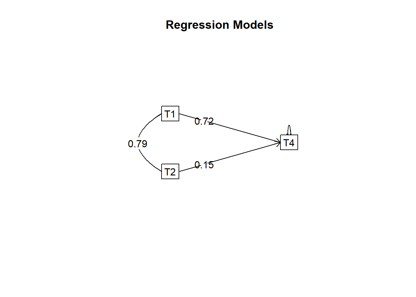
summary(model.cor)
##
## Multiple Regression from matrix input
## setCor(y = "T4", x = c("T1", "T2"), data = cormatlw, n.obs = 18,
##     std = FALSE)
##
## Multiple Regression from matrix input
##
## Beta weights
##      T4
## T1 0.72
## T2 0.15
##
## Multiple R
##      T4
## T4 0.84
##
## Multiple R2
##     T4
## T4 0.7
##
## Cohen's set correlation R2
## [1] 0.7
##
## Squared Canonical Correlations
## NULL