Structural Equation Modeling in R Tutorial 4: Introduction to lavaan using path analysis
Table of Contents
Made for Jonathan Butner’s Structural Equation Modeling Class, Fall 2017, University of Utah. This handout will serve as an introduction to the lavaan package in R, which can be used for structural equation modeling. Mainly, we will focus on how path models can be conducted simply as a series of regressions in the R package lavaan, including estimation of indirect effects with bootstrapping. It will also be briefly reviewed how to fix parameters in lavaan, as well as inspect the underlying matrices of your model. This syntax imports the 4 variable dataset from datafile pathmodel example 3.txt. Note in the comments some additional coding options for things like missing data and standardized estimates.
For more on using lavaan in R, please see the lavaan documentation website. See this page for more on how to run SEM’s in lavaan using simply a covariance matrix if you do not have raw data available.
Data Input
First, we will read in datafile and clean up the datafile a little bit.
library(psych)  #for descriptives
library(lavaan)
library(semPlot)  #for plotting lavaan objects
# make sure to set your working directory to where the file
# is located, e.g. setwd('D:/Downloads/Handout 1 -
# Regression') you can do this in R Studio by going to the
# Session menu - 'Set Working Directory' - To Source File
# Location
socdata <- read.fortran("pathmodel example 3.txt", c("F12.0",
    "3F13.0"))
# note: #The format for a field is of one of the following
# forms: rFl.d, rDl.d, rXl, rAl, rIl, where l is the number
# of columns, d is the number of decimal places, and r is the
# number of repeats. F and D are numeric formats, A is
# character, I is integer, and X indicates columns to be
# skipped. The repeat code r and decimal place code d are
# always optional. The length code l is required except for X
# formats when r is present.

socdata <- read.table("pathmodel example 3.txt")  #this does the same thing as read.fortran above!

# add column names
names(socdata) <- c("Behavior", "Snorm", "Belief", "Intent")

# get descriptives for the data
describe(socdata)
##          vars   n  mean   sd median trimmed  mad   min  max range  skew
## Behavior    1 180  0.09 2.24   0.11    0.12 2.55 -5.85 5.68 11.53 -0.09
## Snorm       2 180 -0.04 2.02   0.02   -0.01 2.03 -5.43 4.23  9.66 -0.13
## Belief      3 180 -0.01 0.96  -0.01    0.01 0.95 -2.40 2.33  4.72 -0.09
## Intent      4 180  0.00 1.01   0.03    0.02 1.02 -3.02 2.06  5.09 -0.29
##          kurtosis   se
## Behavior    -0.27 0.17
## Snorm       -0.31 0.15
## Belief      -0.21 0.07
## Intent      -0.34 0.08
Introduction to Lavaan
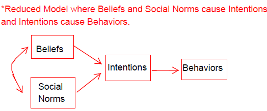
Now, we’ll complete a series of regressions using the lavaan package. First, we will test a reduced model, where beliefs and social norms cause intentions and intentions cause behaviors. If you remember from earlier in class, this is Azjen and Fishbein’s theory of planned behavior.
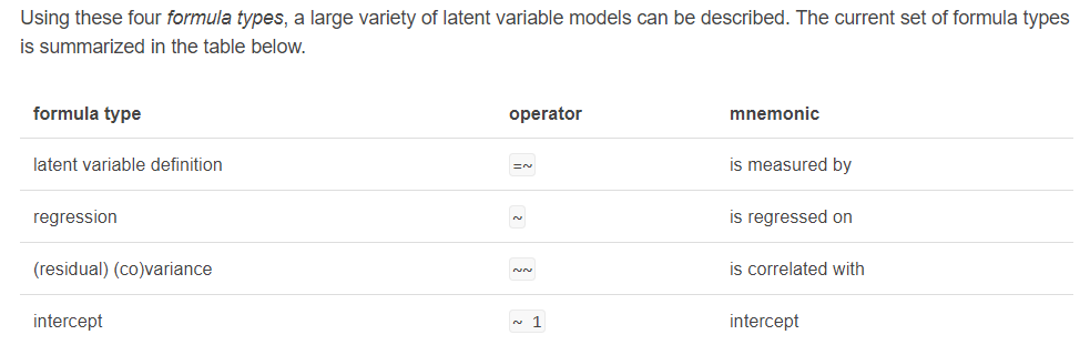
Lavaan syntax is fairly straightforward and parallels MPlus syntax nicely. Note that there are other tricks in lavaan that go beyond the scope of path modeling, but are foreshadowing later parts of the course with more advanced models. Note in the comments below how you can fix parameters using a number and an *. You can also set equality contraints by multiplying two parameters by the same name, such as beta1*Belief + beta1*Snorm.
Note how we are very explicit in the specification of our model, and code the unanalyzed relationship, or correlation, between beliefs and social norms. Lavaan will default to this behavior (correlating exogenous variables), but often it is useful to explicitly specify all parts of the model.
model.reduced <- "Behavior ~ Intent + 0*Snorm
Intent ~ Belief + Snorm
Belief ~~ Snorm
"
# specify our model

# Including '0*' before a variable will fix that relationship
# to 0 (or whatever other number you choose to specify). In
# this example we fixed the casual pathway between belief
# snorm and behavior to 0 (the 2 paths constrained from the
# fully saturated model). However, we can leave out this line
# of code, as lavaan will default to fixing these
# relationships to 0 if we did not ask it to estimate them.

# the estimator = 'ML' tells lavaan to implement maximum
# likelihood estimation. This is the default in lavaan.

# the missing = ML function tells lavaan to treat 'NA' values
# in your dataset as missing and use full information maximum
# likelihood estimation to handle this missingness. Note that
# this should only be used with MAR (missing at random) or
# MCAR (missing completely at random) data.

model.reduced.fit <- sem(model.reduced, estimator = "ML", data = socdata)  #fit our model #add missing = 'ML' for missing data.
summary(model.reduced.fit, fit.measures = TRUE)  #ask R for our results
## lavaan 0.6-5 ended normally after 21 iterations
##
##   Estimator                                         ML
##   Optimization method                           NLMINB
##   Number of free parameters                          8
##
##   Number of observations                           180
##
## Model Test User Model:
##
##   Test statistic                               221.348
##   Degrees of freedom                                 2
##   P-value (Chi-square)                           0.000
##
## Model Test Baseline Model:
##
##   Test statistic                               660.656
##   Degrees of freedom                                 6
##   P-value                                        0.000
##
## User Model versus Baseline Model:
##
##   Comparative Fit Index (CFI)                    0.665
##   Tucker-Lewis Index (TLI)                      -0.005
##
## Loglikelihood and Information Criteria:
##
##   Loglikelihood user model (H0)              -1065.127
##   Loglikelihood unrestricted model (H1)       -954.453
##
##   Akaike (AIC)                                2146.254
##   Bayesian (BIC)                              2171.797
##   Sample-size adjusted Bayesian (BIC)         2146.461
##
## Root Mean Square Error of Approximation:
##
##   RMSEA                                          0.781
##   90 Percent confidence interval - lower         0.696
##   90 Percent confidence interval - upper         0.869
##   P-value RMSEA <= 0.05                          0.000
##
## Standardized Root Mean Square Residual:
##
##   SRMR                                           0.173
##
## Parameter Estimates:
##
##   Information                                 Expected
##   Information saturated (h1) model          Structured
##   Standard errors                             Standard
##
## Regressions:
##                    Estimate  Std.Err  z-value  P(>|z|)
##   Behavior ~
##     Intent            1.566    0.116   13.471    0.000
##     Snorm             0.000
##   Intent ~
##     Belief           -0.317    0.068   -4.654    0.000
##     Snorm             0.495    0.032   15.306    0.000
##
## Covariances:
##                    Estimate  Std.Err  z-value  P(>|z|)
##   Snorm ~~
##     Belief            1.379    0.176    7.830    0.000
##
## Variances:
##                    Estimate  Std.Err  z-value  P(>|z|)
##    .Behavior          2.474    0.261    9.487    0.000
##    .Intent            0.368    0.039    9.487    0.000
##     Snorm             4.046    0.426    9.487    0.000
##     Belief            0.911    0.096    9.487    0.000
# lets use semPlot to plot our results!
semPaths(model.reduced.fit, "par", edge.label.cex = 1.2, fade = FALSE)

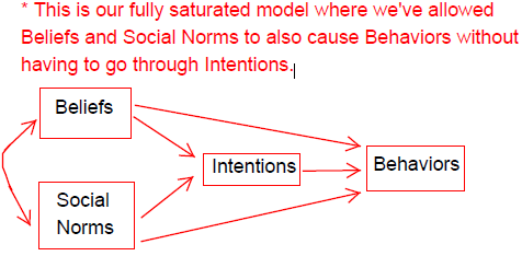
Note how lavaan defaults to certain behaviors sometimes such as estimating intercepts for a path model even though we did not explicily pass that argument to our model. Next, we will run the fully saturated model where we’ve allowed beliefs and social norms to also cause behaviors without having to go through intentions. There will be a final regression that accounts for intentions, social norms, and beliefs all predicting behavior simultaneously. We’ll also calculate the indirect effect between beliefs and behaviors through intentions. Note that we’ll bootstrap standard errors and our test statistics, in order to account for the violation of normality that occurs when multiplying two normal distributions when we create the indirect effect.
model.full <- "Behavior ~ b*Intent + Snorm + Belief
Intent ~ Snorm + a*Belief
Belief ~~ Snorm
Behavior ~ 1
Belief ~ 1
Intent ~ 1
Snorm ~ 1
#calculate indirect effect. a* is where our predictor predicts the mediating variable.
#b* is where our mediator predicts the final dependent variable.
ab := a*b"
# specify our model. note here we explicitly ask for
# intercepts, as opposed to in our previous model
model.full.fit <- sem(model.full, se = "bootstrap", test = "bootstrap",
    data = socdata)  #fit the model to an object
summary(model.full.fit, fit.measures = TRUE)  #ask R for results
## lavaan 0.6-5 ended normally after 24 iterations
##
##   Estimator                                         ML
##   Optimization method                           NLMINB
##   Number of free parameters                         14
##
##   Number of observations                           180
##
## Model Test User Model:
##
##   Test statistic                                 0.000
##   Degrees of freedom                                 0
##
##   Test statistic                                 0.000
##   Degrees of freedom                                 0
##
## Model Test Baseline Model:
##
##   Test statistic                               660.656
##   Degrees of freedom                                 6
##   P-value                                        0.000
##
## User Model versus Baseline Model:
##
##   Comparative Fit Index (CFI)                    1.000
##   Tucker-Lewis Index (TLI)                       1.000
##
## Loglikelihood and Information Criteria:
##
##   Loglikelihood user model (H0)               -954.453
##   Loglikelihood unrestricted model (H1)       -954.453
##
##   Akaike (AIC)                                1936.905
##   Bayesian (BIC)                              1981.607
##   Sample-size adjusted Bayesian (BIC)         1937.269
##
## Root Mean Square Error of Approximation:
##
##   RMSEA                                          0.000
##   90 Percent confidence interval - lower         0.000
##   90 Percent confidence interval - upper         0.000
##   P-value RMSEA <= 0.05                             NA
##
## Standardized Root Mean Square Residual:
##
##   SRMR                                           0.000
##
## Parameter Estimates:
##
##   Standard errors                            Bootstrap
##   Number of requested bootstrap draws             1000
##   Number of successful bootstrap draws            1000
##
## Regressions:
##                    Estimate  Std.Err  z-value  P(>|z|)
##   Behavior ~
##     Intent     (b)    0.019    0.108    0.173    0.863
##     Snorm             0.977    0.068   14.431    0.000
##     Belief            0.116    0.096    1.209    0.227
##   Intent ~
##     Snorm             0.495    0.030   16.740    0.000
##     Belief     (a)   -0.317    0.066   -4.811    0.000
##
## Covariances:
##                    Estimate  Std.Err  z-value  P(>|z|)
##   Snorm ~~
##     Belief            1.379    0.172    8.024    0.000
##
## Intercepts:
##                    Estimate  Std.Err  z-value  P(>|z|)
##    .Behavior          0.126    0.064    1.965    0.049
##     Belief           -0.005    0.068   -0.080    0.936
##    .Intent            0.014    0.043    0.324    0.746
##     Snorm            -0.037    0.145   -0.254    0.799
##
## Variances:
##                    Estimate  Std.Err  z-value  P(>|z|)
##    .Behavior          0.723    0.077    9.369    0.000
##    .Intent            0.368    0.040    9.299    0.000
##     Snorm             4.046    0.379   10.685    0.000
##     Belief            0.911    0.090   10.139    0.000
##
## Defined Parameters:
##                    Estimate  Std.Err  z-value  P(>|z|)
##     ab               -0.006    0.036   -0.165    0.869
# Note that we bootstrap SEs and test statistics as well
# note you can ask for standardized results with the below
# command summary(model.full.fit, fit.measures=TRUE,
# standardized=TRUE)
# the code below bootstraps parameter estimates 500 times
# using multiple processors on your CPU
# model.full.fit.bootstrap <- bootstrapLavaan(model.full.fit,
# R = 500L, parallel = 'multicore')
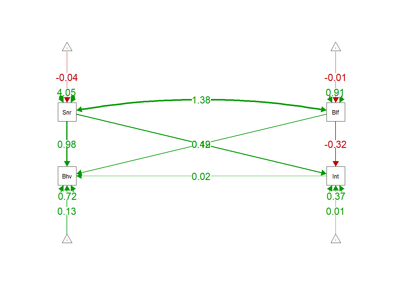
# lets use semPlot to plot our results!
semPaths(model.full.fit, "par", edge.label.cex = 1.2, fade = FALSE)
Inspecting matrices when things go wrong
Sometimes, our model will not converage, standard errors will explode, or psi matrices will not be positive definite. In this case, its often helpful to inspect the matrices underlying your model construction. This is analogous to the “TECH” command in MPlus. In this example we’ll inspect our fully saturated model.
inspect(model.full.fit, "start") #this provides the starting values for parameters
## $lambda
##          Behavr Intent Snorm Belief
## Behavior      1      0     0      0
## Intent        0      1     0      0
## Snorm         0      0     1      0
## Belief        0      0     0      1
##
## $theta
##          Behavr Intent Snorm Belief
## Behavior 0
## Intent   0      0
## Snorm    0      0      0
## Belief   0      0      0     0
##
## $psi
##          Behavr Intent Snorm Belief
## Behavior 2.484
## Intent   0.000  0.508
## Snorm    0.000  0.000  2.023
## Belief   0.000  0.000  0.000 0.455
##
## $beta
##          Behavr Intent Snorm Belief
## Behavior      0      0     0      0
## Intent        0      0     0      0
## Snorm         0      0     0      0
## Belief        0      0     0      0
##
## $nu
##          intrcp
## Behavior      0
## Intent        0
## Snorm         0
## Belief        0
##
## $alpha
##          intrcp
## Behavior  0.089
## Intent   -0.002
## Snorm    -0.037
## Belief   -0.005
inspect(model.full.fit, "free") #this provides the parameters that are free
## $lambda
##          Behavr Intent Snorm Belief
## Behavior      0      0     0      0
## Intent        0      0     0      0
## Snorm         0      0     0      0
## Belief        0      0     0      0
##
## $theta
##          Behavr Intent Snorm Belief
## Behavior 0
## Intent   0      0
## Snorm    0      0      0
## Belief   0      0      0     0
##
## $psi
##          Behavr Intent Snorm Belief
## Behavior 11
## Intent    0     12
## Snorm     0      0     13
## Belief    0      0      6    14
##
## $beta
##          Behavr Intent Snorm Belief
## Behavior      0      1     2      3
## Intent        0      0     4      5
## Snorm         0      0     0      0
## Belief        0      0     0      0
##
## $nu
##          intrcp
## Behavior      0
## Intent        0
## Snorm         0
## Belief        0
##
## $alpha
##          intrcp
## Behavior      7
## Intent        9
## Snorm        10
## Belief        8
# (in other words, the parameters that are estimated)
Modeling in Lavaan Using a Covariance Matrix
Imagine that you’re interesting in conducting follow-up analyses on another researcher’s manuscript, but only have access to their covariance matrix, which was provided in an appendix. You’ll sometimes not have access to raw data, and instead want to run a lavaan model using a covariance matrix input. The following code shows how this differs from specifying a model with raw data, as is shown previously.
socdata.cov <- cov(socdata)  #this time we'll just pull the covariance matrix from our data
# as a demonstration. But note that sometimes covariance
# matrices are published and so you can simply manually enter
# them.
socdata.cov  #will print covariance matrix.
##          Behavior    Snorm    Belief    Intent
## Behavior 4.996093 4.164750 1.4687772 1.6014688
## Snorm    4.164750 4.068619 1.3871273 1.5729111
## Belief   1.468777 1.387127 0.9156302 0.3958586
## Intent   1.601469 1.572911 0.3958586 1.0225483
# you can just copy paste this into the model and delete the
# upper triangle values. assigns to object that lavaan will
# understand
lower <- "4.996093
          4.164750 4.068619
          1.468777 1.387127 0.9156302
          1.601469 1.572911 0.3958586 1.0225483"
# convert to a full symmetric covariance matrix with names
test.cov <- getCov(lower, names = c("Behavior", "Snorm", "Belief",
    "Intent"))
# reproduce the fully saturated model from earlier
model.fromcov <- "Behavior ~ b*Intent + Snorm + Belief
Intent ~ Snorm + a*Belief
Belief ~~ Snorm
Behavior ~ 1
Belief ~ 1
Intent ~ 1
Snorm ~ 1
#calculate indirect effect. a* is where our predictor predicts the mediating variable.
#b* is where our mediator predicts the final dependent variable.
ab := a*b"
fit.fromcov <- sem(model.fromcov, sample.cov = test.cov, sample.nobs = 180)
summary(fit.fromcov)
## lavaan 0.6-5 ended normally after 23 iterations
##
##   Estimator                                         ML
##   Optimization method                           NLMINB
##   Number of free parameters                         14
##
##   Number of observations                           180
##
## Model Test User Model:
##
##   Test statistic                                 0.000
##   Degrees of freedom                                 0
##
## Parameter Estimates:
##
##   Information                                 Expected
##   Information saturated (h1) model          Structured
##   Standard errors                             Standard
##
## Regressions:
##                    Estimate  Std.Err  z-value  P(>|z|)
##   Behavior ~
##     Intent     (b)    0.019    0.105    0.178    0.858
##     Snorm             0.977    0.069   14.206    0.000
##     Belief            0.116    0.101    1.150    0.250
##   Intent ~
##     Snorm             0.495    0.032   15.306    0.000
##     Belief     (a)   -0.317    0.068   -4.654    0.000
##
## Covariances:
##                    Estimate  Std.Err  z-value  P(>|z|)
##   Snorm ~~
##     Belief            1.379    0.176    7.830    0.000
##
## Intercepts:
##                    Estimate  Std.Err  z-value  P(>|z|)
##    .Behavior          0.000    0.063    0.000    1.000
##     Belief            0.000    0.071    0.000    1.000
##    .Intent            0.000    0.045    0.000    1.000
##     Snorm             0.000    0.150    0.000    1.000
##
## Variances:
##                    Estimate  Std.Err  z-value  P(>|z|)
##    .Behavior          0.723    0.076    9.487    0.000
##    .Intent            0.368    0.039    9.487    0.000
##     Snorm             4.046    0.426    9.487    0.000
##     Belief            0.911    0.096    9.487    0.000
##
## Defined Parameters:
##                    Estimate  Std.Err  z-value  P(>|z|)
##     ab               -0.006    0.033   -0.178    0.859
And, magically, we exactly replicate our results from the earlier model computed using raw data. This is because SEM always does calculations using the correlation and/or covariance matrices rather than raw data.
Ian Ruginski
Postdoctoral Fellow
My research interests include spatial cognition, navigation, data visualization, and human-computer interaction.