Structural Equation Modeling in R Tutorial 7: Full Structural Equation Modeling
Table of Contents
Made for Jonathan Butner’s Structural Equation Modeling Class, Fall 2017, University of Utah. This handout begins by showing how to import a matrix into R. Then, we will overview how to establish a measurement model in R using the lavaan package. As we go, I’ll demonstrate how to quickly and easily plot the results of your confirmatory factor analysis using semPlot. ast, I’ll demonstrate how to do basic model comparisons using lavaan objects, which will help to inform decisions related to which model fits your data better. This syntax imports the 14 variable, 307 person dataset called EXMP8MATRIX.txt, which is a free format text file. The data are for 13 observed variables comprising three theorized latent factors (Socioeconomic Status, Communication, and Conduct), as well as biological sex, dummy coded as 0 or 1, where 0 is female and 1 is male. There is no missing data.
Data Input
First, we will read in the datafile and clean up the datafile a little bit, as well as load required packages.
library(lavaan)  #for doing the CFA
library(semPlot)  #for plotting your CFA
library(dplyr)  #for subsetting data quickly if needed

# make sure to set your working directory to where the file
# is located, e.g. setwd('D:/Downloads/Handout 1 -
# Regression') you can do this in R Studio using menus by
# going to the Session menu - 'Set Working Directory' - To
# Source File Location
semdat <- read.table("EXMP8MATRIX.txt")
# note that this data is in free format so we use read.table

# add column names
names(semdat) <- c("Sex", "Pa_Ed", "Ma_Ed", "Pa_Occ", "Ma_Occ",
    "Income", "Accept", "Listen", "Commun", "Openness", "Patience",
    "Act_Out", "Agress", "Hostile")
head(semdat)  #take a look at the beginning of our datafile
##   Sex Pa_Ed Ma_Ed Pa_Occ Ma_Occ Income Accept Listen Commun Openness
## 1   0 -0.28  0.54   1.27   0.06   1.58   1.46   1.88   2.86     0.48
## 2   0 -0.26  0.02  -0.67   0.20  -0.15   0.84   0.62  -1.06     0.22
## 3   0 -0.61 -0.01  -0.05  -0.85  -0.04   0.85   0.11  -0.07     0.36
## 4   0 -0.67 -2.26   0.45   0.16   0.43   0.12  -0.37  -0.57    -1.93
## 5   0 -0.35 -1.05   0.22   0.57  -0.63   0.14  -0.36   0.36     1.14
## 6   0  1.85 -0.90   0.97  -0.19   0.86  -0.47   1.23   0.99     0.46
##   Patience Act_Out Agress Hostile
## 1     2.00   -2.78  -2.71   -1.85
## 2     1.21   -3.07  -2.09   -1.40
## 3     0.07   -1.19  -0.52   -1.48
## 4    -0.43    0.46  -1.22   -0.26
## 5    -0.06   -2.39  -1.63    2.26
## 6    -0.11    0.37  -0.57   -1.47
Structural Equation Modeling Using lavaan: Measurement Model
Typically the first step in structural equation modeing is to establish what’s called a “measurement model”, a model which includes all of your observed variables that are going to be represented with latent variables. Constructing a measurement model allows to determine model fit related to the latent portion of your model. This way you can more precisely know where model misfit is most prevalent in your model.
Remember that * fixes variables to a particular value. Here we adopt the marker variable identification approach, where we fix the loading of one indicator in each latent to 1 in order to identify the model and give each latent factor a metric. This will not change model fit, just some of the loadings in the model. This makes it so that a one unit change in the latent factor is interpreted as a unit unit change in the scale of the observed variable selected as the marker variable (the variable loading we fix to 1). Note also that variances and disturbances (errors) are estimated by default.
sem.model.measurement <- "SES =~ 1*Pa_Ed + Ma_Ed + Pa_Occ + Ma_Occ + Income
#make 5 indicator latent socioeconomic status (SES) factor with parents education variable as the marker
COM =~ 1*Accept + Listen + Commun + Openness + Patience
#make 5 indicator latent communication factor with accept variable as the marker
Conduct =~ 1*Act_Out + Agress + Hostile
#make 3 indicator latent conduct factor with acting out variable as the marker"

sem.fit.measurement <- sem(sem.model.measurement, data = semdat)
summary(sem.fit.measurement, fit.measures = TRUE)
## lavaan 0.6-5 ended normally after 34 iterations
##
##   Estimator                                         ML
##   Optimization method                           NLMINB
##   Number of free parameters                         29
##
##   Number of observations                           307
##
## Model Test User Model:
##
##   Test statistic                               120.948
##   Degrees of freedom                                62
##   P-value (Chi-square)                           0.000
##
## Model Test Baseline Model:
##
##   Test statistic                              1403.563
##   Degrees of freedom                                78
##   P-value                                        0.000
##
## User Model versus Baseline Model:
##
##   Comparative Fit Index (CFI)                    0.956
##   Tucker-Lewis Index (TLI)                       0.944
##
## Loglikelihood and Information Criteria:
##
##   Loglikelihood user model (H0)              -5835.118
##   Loglikelihood unrestricted model (H1)      -5774.644
##
##   Akaike (AIC)                               11728.236
##   Bayesian (BIC)                             11836.314
##   Sample-size adjusted Bayesian (BIC)        11744.339
##
## Root Mean Square Error of Approximation:
##
##   RMSEA                                          0.056
##   90 Percent confidence interval - lower         0.041
##   90 Percent confidence interval - upper         0.070
##   P-value RMSEA <= 0.05                          0.251
##
## Standardized Root Mean Square Residual:
##
##   SRMR                                           0.049
##
## Parameter Estimates:
##
##   Information                                 Expected
##   Information saturated (h1) model          Structured
##   Standard errors                             Standard
##
## Latent Variables:
##                    Estimate  Std.Err  z-value  P(>|z|)
##   SES =~
##     Pa_Ed             1.000
##     Ma_Ed             1.457    0.144   10.144    0.000
##     Pa_Occ            1.245    0.130    9.559    0.000
##     Ma_Occ            0.896    0.101    8.893    0.000
##     Income            0.876    0.113    7.776    0.000
##   COM =~
##     Accept            1.000
##     Listen            0.811    0.067   12.035    0.000
##     Commun            1.132    0.095   11.937    0.000
##     Openness          0.602    0.070    8.609    0.000
##     Patience          0.737    0.079    9.298    0.000
##   Conduct =~
##     Act_Out           1.000
##     Agress            0.752    0.073   10.305    0.000
##     Hostile           0.893    0.082   10.842    0.000
##
## Covariances:
##                    Estimate  Std.Err  z-value  P(>|z|)
##   SES ~~
##     COM               0.467    0.070    6.645    0.000
##     Conduct          -0.223    0.061   -3.659    0.000
##   COM ~~
##     Conduct          -0.487    0.088   -5.528    0.000
##
## Variances:
##                    Estimate  Std.Err  z-value  P(>|z|)
##    .Pa_Ed             0.837    0.077   10.856    0.000
##    .Ma_Ed             0.642    0.079    8.108    0.000
##    .Pa_Occ            0.762    0.078    9.737    0.000
##    .Ma_Occ            0.580    0.055   10.609    0.000
##    .Income            0.950    0.084   11.361    0.000
##    .Accept            0.786    0.082    9.541    0.000
##    .Listen            0.480    0.052    9.317    0.000
##    .Commun            0.976    0.103    9.449    0.000
##    .Openness          0.876    0.076   11.480    0.000
##    .Patience          1.050    0.093   11.249    0.000
##    .Act_Out           0.723    0.108    6.697    0.000
##    .Agress            0.817    0.085    9.601    0.000
##    .Hostile           0.740    0.094    7.833    0.000
##     SES               0.510    0.093    5.488    0.000
##     COM               0.960    0.136    7.037    0.000
##     Conduct           1.231    0.172    7.139    0.000
semPaths(sem.fit.measurement, "par", edge.label.cex = 1.2, fade = FALSE) #plot our CFA
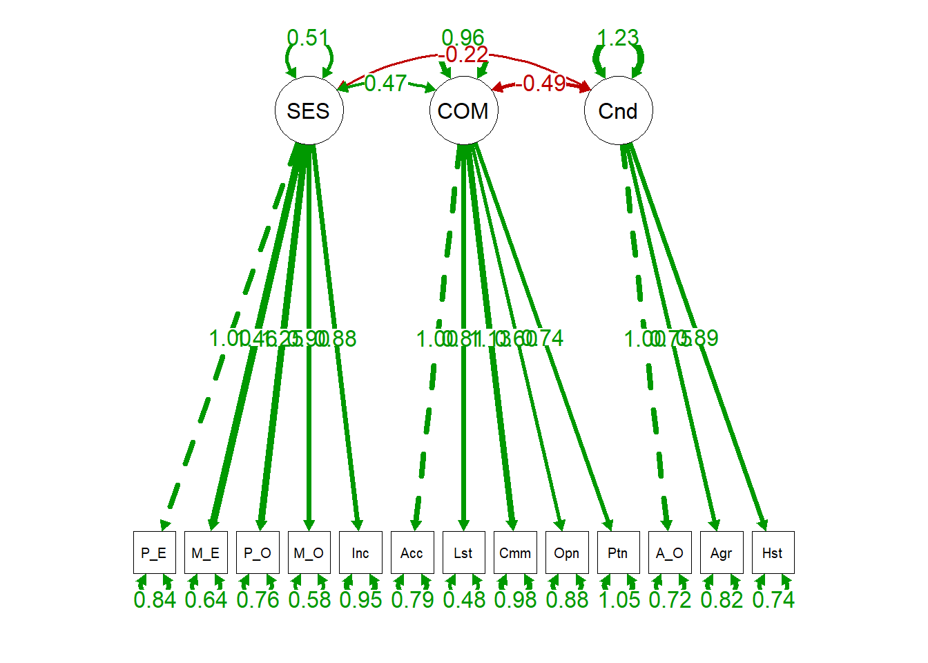
In the figure, you can see the marker variables that we fixed to one as well as how each of the other observed variables loads onto each latent factor.From this model output, we can see that our fit is pretty good (CFI/TLI around .95, RMSEA approaching .05, SRMR < .05).
Structural Equation Modeling Using lavaan: Full Model
Now, we will estimate a full model that includes predictive components in addition to measurement components. We will still use the marker variable approach, making the measurement model portion of our model unchanged.
sem.model.full <- "SES =~ 1*Pa_Ed + Ma_Ed + Pa_Occ + Ma_Occ + Income #make 5 indicator latent socioeconomic status (SES) factor with parents education variable as the marker
             COM =~ 1*Accept + Listen + Commun + Openness + Patience; #make 5 indicator latent communication factor with accept variable as the marker
            Conduct =~ 1*Act_Out + Agress + Hostile #make 3 indicator latent conduct factor with acting out variable as the marker
COM ~ Sex + SES #Regress COM on Sex and SES
Conduct ~ Sex + COM #Regress Conduct on Sex and COM
"

sem.fit.full <- sem(sem.model.full, data = semdat)
summary(sem.fit.full, fit.measures = TRUE)  #ask for model results
## lavaan 0.6-5 ended normally after 32 iterations
##
##   Estimator                                         ML
##   Optimization method                           NLMINB
##   Number of free parameters                         30
##
##   Number of observations                           307
##
## Model Test User Model:
##
##   Test statistic                               143.535
##   Degrees of freedom                                74
##   P-value (Chi-square)                           0.000
##
## Model Test Baseline Model:
##
##   Test statistic                              1486.134
##   Degrees of freedom                                91
##   P-value                                        0.000
##
## User Model versus Baseline Model:
##
##   Comparative Fit Index (CFI)                    0.950
##   Tucker-Lewis Index (TLI)                       0.939
##
## Loglikelihood and Information Criteria:
##
##   Loglikelihood user model (H0)              -5805.126
##   Loglikelihood unrestricted model (H1)      -5733.359
##
##   Akaike (AIC)                               11670.252
##   Bayesian (BIC)                             11782.058
##   Sample-size adjusted Bayesian (BIC)        11686.911
##
## Root Mean Square Error of Approximation:
##
##   RMSEA                                          0.055
##   90 Percent confidence interval - lower         0.042
##   90 Percent confidence interval - upper         0.069
##   P-value RMSEA <= 0.05                          0.247
##
## Standardized Root Mean Square Residual:
##
##   SRMR                                           0.053
##
## Parameter Estimates:
##
##   Information                                 Expected
##   Information saturated (h1) model          Structured
##   Standard errors                             Standard
##
## Latent Variables:
##                    Estimate  Std.Err  z-value  P(>|z|)
##   SES =~
##     Pa_Ed             1.000
##     Ma_Ed             1.479    0.146   10.154    0.000
##     Pa_Occ            1.246    0.131    9.492    0.000
##     Ma_Occ            0.907    0.102    8.910    0.000
##     Income            0.875    0.113    7.717    0.000
##   COM =~
##     Accept            1.000
##     Listen            0.807    0.066   12.160    0.000
##     Commun            1.131    0.093   12.104    0.000
##     Openness          0.604    0.069    8.756    0.000
##     Patience          0.740    0.078    9.462    0.000
##   Conduct =~
##     Act_Out           1.000
##     Agress            0.739    0.068   10.900    0.000
##     Hostile           0.877    0.074   11.782    0.000
##
## Regressions:
##                    Estimate  Std.Err  z-value  P(>|z|)
##   COM ~
##     Sex              -0.311    0.105   -2.971    0.003
##     SES               0.955    0.119    7.994    0.000
##   Conduct ~
##     Sex               0.904    0.133    6.789    0.000
##     COM              -0.485    0.076   -6.377    0.000
##
## Variances:
##                    Estimate  Std.Err  z-value  P(>|z|)
##    .Pa_Ed             0.844    0.077   10.924    0.000
##    .Ma_Ed             0.626    0.078    8.026    0.000
##    .Pa_Occ            0.772    0.078    9.865    0.000
##    .Ma_Occ            0.575    0.054   10.611    0.000
##    .Income            0.956    0.084   11.405    0.000
##    .Accept            0.788    0.082    9.587    0.000
##    .Listen            0.487    0.052    9.437    0.000
##    .Commun            0.980    0.103    9.507    0.000
##    .Openness          0.874    0.076   11.482    0.000
##    .Patience          1.046    0.093   11.250    0.000
##    .Act_Out           0.695    0.100    6.982    0.000
##    .Agress            0.826    0.083    9.936    0.000
##    .Hostile           0.753    0.089    8.450    0.000
##     SES               0.503    0.092    5.453    0.000
##    .COM               0.498    0.083    6.026    0.000
##    .Conduct           0.803    0.119    6.741    0.000
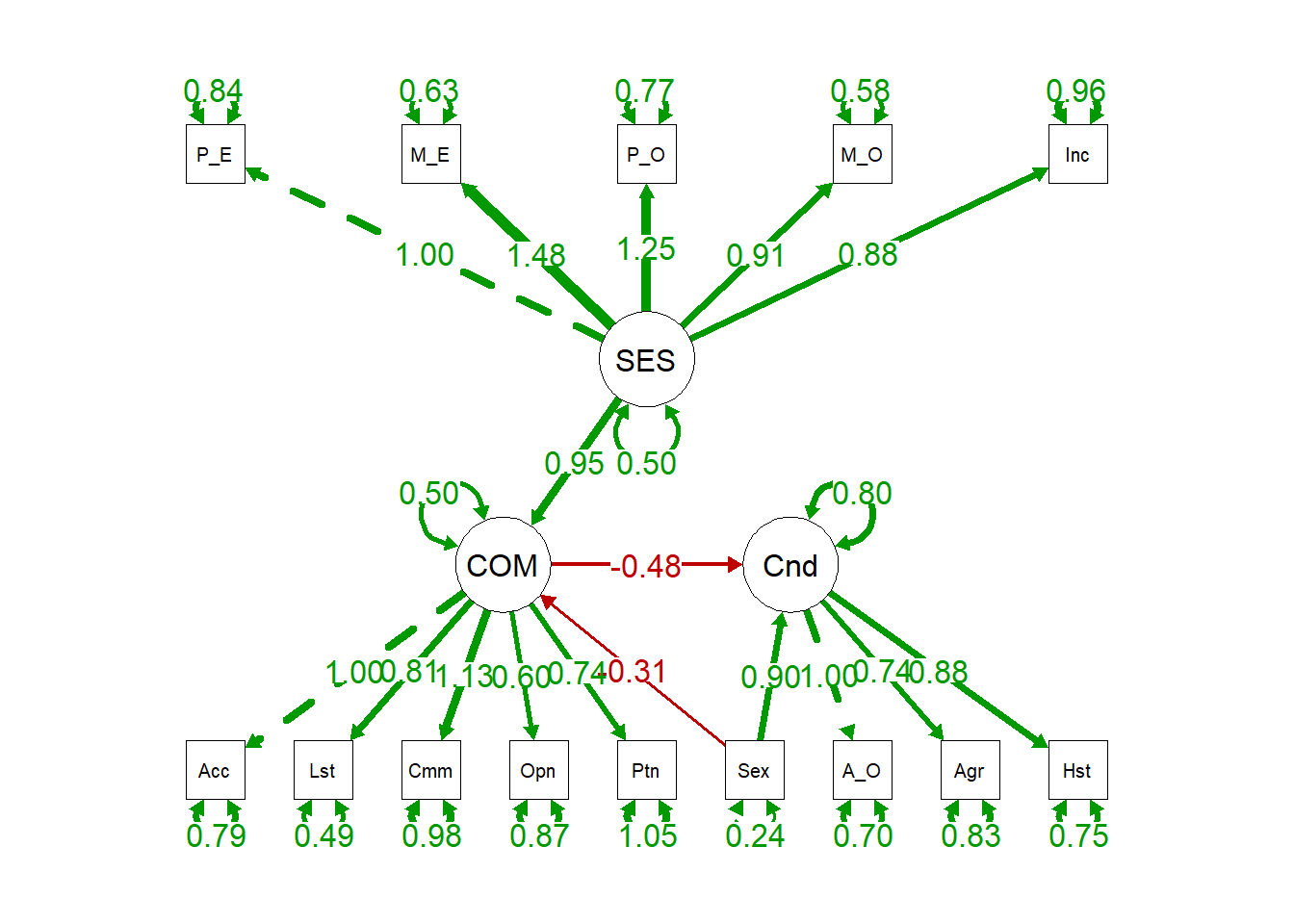
semPaths(sem.fit.full, "par", edge.label.cex = 1.2, fade = FALSE) #plot our CFA. you can change layout with layout = argument. see ?semPaths() for more.
Next, we’ll estimated an alternative, more saturated model that has one additional parameter estimated: the path between SES and conduct, with SES predicting Conduct. Essentially, we add an additional predictor in our regression, whereas that parameter was fixed to 0 in our previous model.
sem.model.full.1free <- "SES =~ 1*Pa_Ed + Ma_Ed + Pa_Occ + Ma_Occ + Income #make 5 indicator latent socioeconomic status (SES) factor with parents education variable as the marker
             COM =~ 1*Accept + Listen + Commun + Openness + Patience; #make 5 indicator latent communication factor with accept variable as the marker
            Conduct =~ 1*Act_Out + Agress + Hostile #make 3 indicator latent conduct factor with acting out variable as the marker
COM ~ Sex + SES #Regress COM on Sex and SES
Conduct ~ Sex + COM + SES #Regress Conduct on Sex, COM, and SES
"
sem.fit.full.1free <- sem(sem.model.full.1free, data = semdat)
summary(sem.fit.full.1free, fit.measures = TRUE)
## lavaan 0.6-5 ended normally after 34 iterations
##
##   Estimator                                         ML
##   Optimization method                           NLMINB
##   Number of free parameters                         31
##
##   Number of observations                           307
##
## Model Test User Model:
##
##   Test statistic                               142.417
##   Degrees of freedom                                73
##   P-value (Chi-square)                           0.000
##
## Model Test Baseline Model:
##
##   Test statistic                              1486.134
##   Degrees of freedom                                91
##   P-value                                        0.000
##
## User Model versus Baseline Model:
##
##   Comparative Fit Index (CFI)                    0.950
##   Tucker-Lewis Index (TLI)                       0.938
##
## Loglikelihood and Information Criteria:
##
##   Loglikelihood user model (H0)              -5804.567
##   Loglikelihood unrestricted model (H1)      -5733.359
##
##   Akaike (AIC)                               11671.134
##   Bayesian (BIC)                             11786.666
##   Sample-size adjusted Bayesian (BIC)        11688.348
##
## Root Mean Square Error of Approximation:
##
##   RMSEA                                          0.056
##   90 Percent confidence interval - lower         0.042
##   90 Percent confidence interval - upper         0.069
##   P-value RMSEA <= 0.05                          0.236
##
## Standardized Root Mean Square Residual:
##
##   SRMR                                           0.054
##
## Parameter Estimates:
##
##   Information                                 Expected
##   Information saturated (h1) model          Structured
##   Standard errors                             Standard
##
## Latent Variables:
##                    Estimate  Std.Err  z-value  P(>|z|)
##   SES =~
##     Pa_Ed             1.000
##     Ma_Ed             1.480    0.146   10.162    0.000
##     Pa_Occ            1.242    0.131    9.475    0.000
##     Ma_Occ            0.909    0.102    8.924    0.000
##     Income            0.876    0.113    7.720    0.000
##   COM =~
##     Accept            1.000
##     Listen            0.810    0.066   12.221    0.000
##     Commun            1.130    0.093   12.109    0.000
##     Openness          0.600    0.069    8.709    0.000
##     Patience          0.738    0.078    9.448    0.000
##   Conduct =~
##     Act_Out           1.000
##     Agress            0.741    0.068   10.970    0.000
##     Hostile           0.875    0.074   11.822    0.000
##
## Regressions:
##                    Estimate  Std.Err  z-value  P(>|z|)
##   COM ~
##     Sex              -0.309    0.105   -2.945    0.003
##     SES               0.948    0.119    7.944    0.000
##   Conduct ~
##     Sex               0.945    0.136    6.969    0.000
##     COM              -0.390    0.113   -3.459    0.001
##     SES              -0.165    0.153   -1.079    0.281
##
## Variances:
##                    Estimate  Std.Err  z-value  P(>|z|)
##    .Pa_Ed             0.844    0.077   10.928    0.000
##    .Ma_Ed             0.623    0.078    8.009    0.000
##    .Pa_Occ            0.777    0.078    9.902    0.000
##    .Ma_Occ            0.573    0.054   10.602    0.000
##    .Income            0.956    0.084   11.407    0.000
##    .Accept            0.785    0.082    9.544    0.000
##    .Listen            0.480    0.051    9.330    0.000
##    .Commun            0.979    0.103    9.474    0.000
##    .Openness          0.877    0.076   11.489    0.000
##    .Patience          1.048    0.093   11.247    0.000
##    .Act_Out           0.694    0.099    6.986    0.000
##    .Agress            0.822    0.083    9.915    0.000
##    .Hostile           0.757    0.089    8.508    0.000
##     SES               0.503    0.092    5.453    0.000
##    .COM               0.507    0.084    6.041    0.000
##    .Conduct           0.808    0.119    6.793    0.000
semPaths(sem.fit.full.1free, "par", edge.label.cex = 1.2, fade = FALSE) #plot our CFA
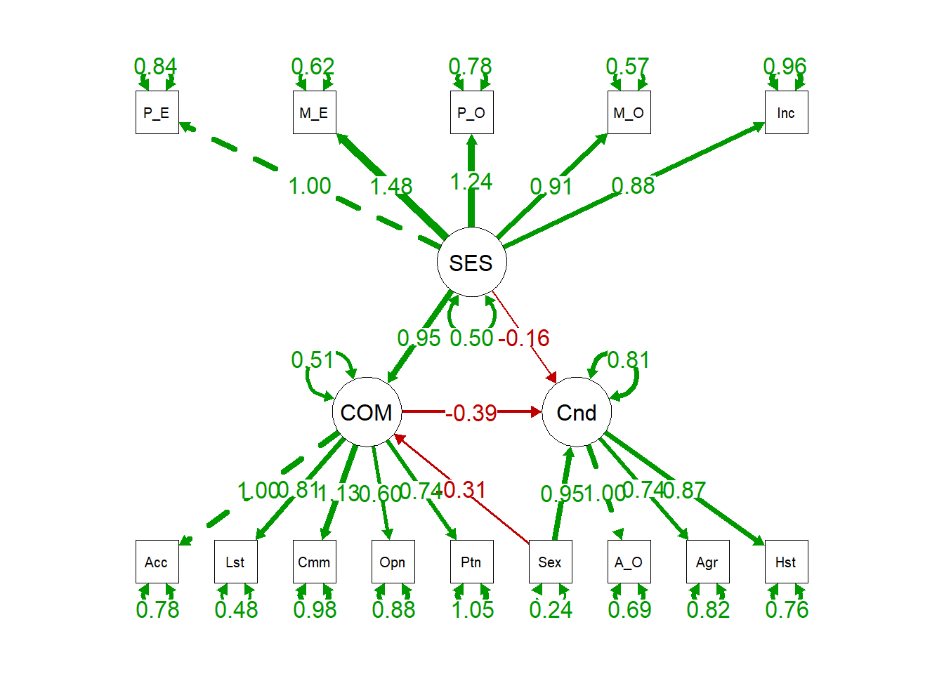
Note how the effect of SES on Conduct is fairly weak (-.16 unstandardized, not significantly different from 0 ,p = 0.28). In addition, fit appears to have worsened (CFI/TLI are smaller, RMSEA/SRMR are larger), but we can explicitly quantitatively test this using the Chi-squared difference of fit test since the models are nested (more on that later), which we will do in the next section.
Model Comparison Using lavaan
Note that models that are compared using most fit statistics must be nested in order for the tests to be valid. Nested models are models that contain at least all of the same exact observed variables contained in the less complicated model. For nested models, you can only free or fix parameter(s), not do both. The underlying data matrix must be the exact same between models. The code below compares the reduced model with more df (regression between Conduct and SES fixed to 0) to the more saturated model with one less df (regression between Conduct and SES estimated).
anova(sem.fit.full, sem.fit.full.1free) #model fit comparison
## Chi-Squared Difference Test
##
##                    Df   AIC   BIC  Chisq Chisq diff Df diff Pr(>Chisq)
## sem.fit.full.1free 73 11671 11787 142.42
## sem.fit.full       74 11670 11782 143.54     1.1182       1     0.2903
Since we retain the null hypothesis using the chi-squared difference of fit test, this means that the less saturated model with one less parameter estimated (in this case, when the regression between Conduct and SES is fixed to 0) fits the data better than the more free model with that regression coefficient estimated. Specifically, the previous model chi-square was 139.486, DF=73, the change between the two is 139.486-138.345=1.141, DF=73-72=1, cutoff value in a chi-squared distribution for 1 df is 3.84 at p=.05. we retain the null thus the new model wth an additional parameter estimated is not a significant improvement over the first more restricted model where that parameter was fixed to 0.
Interpreting and Writing Up Your Model
Congratulations! You’ve just fun your first full SEM model and compared two models, settling on a model that is more plausible given model fit comparison. However, what about intepreting your final model? Interpreting mostly mirrors typical regression, where you can discuss one unit increases in your predictor leading to a beta coefficient increase or decrease in your outcome. From the full, better model above, for example, you would claim that a one unit change in Sex leads to a .90 increase in conduct while controlling for communication. Put more siimply considering dummy coding, men (1) have .9 higher conduct scores than women (0) controlling for communication. Latent variables that are predictors in regression equations follow the same rules, but keep in mind hte metric that you have set for the latent variable (how you chose to identify your latents) when interpreting. If you chose the factor variance identification approach, where you constrained the variance of the latent variable to 1, you will discuss interpretation in terms of one standard deviation changes in that latent variable. If you chose the marker variable identification approach, where you constrained the loading of one of your observed variables comprising your latent variable to 1, you discuss interpretation in terms of one unit changes in the metric of the marker variable. Since we chose the marker variable approach in our full model above, we would say that a one likert (the scale of acceptance, the marker) change in communication leads to a .485 decrease in conduct while controlling for sex.
Ian Ruginski
Postdoctoral Fellow
My research interests include spatial cognition, navigation, data visualization, and human-computer interaction.